On the 12th-14th of June I will be delivering the newly styled and updated Data Vault implementation and automation training together with Doerffler & Partner. I am really looking forward to continue the collaboration after last year’s awesome Data Vault Day (organised by Doerffler as well). Working really hard to wrap up the next layer of virtualisation to discuss there and I’m really excited about it: imagine having multiple versions of not only the Data Marts but the entire Data Warehouse active at a single point in time!

If you’re in or near to Germany, give have a look at the new website: http://www.datavault.de/.

In the meantime wrapping up an extremely busy period with lots of travel, but plenty of new inspiration to write some new posts soon.

When changes are just too many

When you construct a Point-In-Time (PIT) table or Dimension from your Data Vault model, do you sometimes find yourself in the situation where there are too many change records present? This is because, in the standard Data Vault design, tiny variations when loading data may result in the creation of very small time slices when the various historised data sets (e.g. Satellites) are combined.

There is such a thing as too much information, and this post explains ways to remediate this by applying various ‘time condensing’ mechanism. Applying these techniques can have a significant impact on the performance and ease-of-maintenance for PIT and Dimension tables, and is worth looking into.

This post builds on some of the concepts that were covered in earlier posts. Please have a look at the following follow fundamental concepts first, or alternatively meet me at the Data Vault Implementation training at http://www.datavault.de to discuss in person :-). The main relevant concepts are:

• When is a change a change? This post outlines the concepts and effects of row condensing, and why these types of additional checks are needed to avoid record sets with (potentially) many redundant rows.
• Row condensing for Satellites. This posts explains how row condensing works in its most elaborate form.
• Creation of Point-In-Time (PIT) tables. This posts covers the merging of multiple time-variant (historised) data sets to create a full view of history.

When new data is loaded as part of a Data Vault architecture, every record is time-stamped upon entry with the ‘Load Date/Time Stamp‘ (LDTS). This approach ensure a consistent way of ‘effective dating’ data in a way that is fully within the control of the Data Warehouse environment (e.g. cannot be impacted by how OLTP systems behave).

By using this Load Date/Time Stamp as effective date in the Data Vault model, you contribute significantly to ensuring the ‘back-room’ of the Data Warehouse / ETL ‘just works’ so you can concentrate on the ‘front-room’ where most of the business logic is applied.

The very reason that the Load Date/Time Stamp is the effective date in Satellites means that the time when the interface picks up new changes from the source systems is relevant. In other words, the order in which interfaces are received. This should not be confused with the implementation of parallelism and independent loading, as it is still perfectly possible to absorb data in any order of loading. The initial point I want to make is that even though data can be received and processed in a different order (e.g. independent), there are still effects to be aware of in terms of ETL behaviour.

Side effects of independent loading patterns

For instance if you receive a transaction for a purchase (unoriginally called ‘Purchase Transaction’ here) that includes a customer identifier (Customer ID) and some transaction information, you will be able to fully load this information even for the relationship to the Customer. This is because the Customer ID will generate a new Hub record (assuming this is the Business Key and the specific Customer ID didn’t yet exist) even though nothing else is known about the customer. If, a bit later, the Customer Details become available the same Customer ID will be presented to the Hub. But in this case no new key is created since the key already is present, it was delivered by the Purchase Transaction data. The additional context data such as for instance Name, Date of Birth etc. will be loaded to a Satellite as normal. The end result is that a transaction is created and linked to a customer (key) which has certain context attributes.

When the files are received the other way around the end result in terms of available data is the same. That is, the Customer key is created, the context attributes are available for that key and relationships to transactions would have been created. However, in this scenario the Customer Details will be the first to present the Customer ID and will trigger the creation of the Hub record (and the Satellite will be loaded as per usual again). When the Purchase  Transaction is presented to the Data Warehouse, it will detect that the Customer ID is already present and will not create a new Hub record. This is BAU for the Data Warehouse, but the point I’m trying to make is that the Load Date/Time Stamps will be different. And this has an impact when you combine the tables into a single time-variant data set as is the case with a PIT or Dimension.

Consider the following example:

In this small example you can already see that combining information into a single (time-variant) set will produce different results because of the tiny difference in receiving the data (look at the Load Date Time Stamp). From a ‘time’ perspective (for the temporal purists: along the perspective of the LDTS) the finished ETL will produce the following results:

Why wouldn’t you just leave the Hub date/time out of the selection, you may think? Please consider this is a simple example to show the behaviour of the ETL in combination with the Load Date/Time Stamp approach. We’re still investigating the pattern.

This effect is multiplied when you consider multiple sources of information being combined around the ‘Customer’ business concept as in the following example.

Because it is very likely that the above three source tables are presented to the Data Warehouse at slightly different intervals there will be minute (tiny) differences which, while not visible in the individual Satellites, will create NULL values in the combined time-variant result. Again, this should be considered BAU for the Data Warehouse. Works as intended. Have a look at the following example output, considering that -even though these workflows run independently- the data from the source tables arrives in the following order:

1. Customer Email (at 2017-06-05 09:10)
2. Customer Address (at 2017-06-05 09:25)
3. Customer Details (at 2017-06-06 09:26)

This translates into the following behaviour and results when combining the three time-variant / historised sets (Satellites).

At this stage I need to add a disclaimer for some of the temporal purists around: this is the effect that happens when you choose to continue the Load Date / Time Stamp as (Satellite) Effective Date from your Data Vault model into the next layer. Of course, you have the option to choose any other timeline (=available attribute) to represent data against. But for all intends and purposes the standard Load Date / Time Stamp is considered ‘cookie cutter’ for this article.

Condensing changes, over time

As the above example highlights that, in general, the more time-variant data sets you combine the smaller the time slices will become and consequently the more records you will have in your result.

The approaches covering parallelism and independent loading briefly outlined here support a wide range of options to manage the Data Warehouse and ETL environment in a flexible and robust way. Data Vault intends to support ‘100% of the data 100% of the time’, but as a side effect there may be sometimes too many changes available when the complete view is presented back to the user. Especially when adding the effect these minute timing differences have on the size of the record set.

Is the user really interested in seeing that it took a millisecond for address data and email address to be added, that there was a tiny moment that the email wasn’t available yet? For longer periods maybe, but these changes are directed by technical behaviour. Another way of thinking about this is that while there may definitely be functional requirements to show less rows, there is definitely a technical consideration as well.

So, minute timing differences will create new rows. This is expensive, and may not be required. To counter this additional layers of ‘time condensing’ can be applied and used in conjunction with the already required record condensing mechanism – something that every time-variant merge needs.

Time-condensing is different than record condensing. Record condensing focuses on removing redundant rows from the record set (e.g. different time, but no change in values), while time condensing is about removing rows (and keeping one) from a defined period of time even if they are genuine changes (the values are different across rows). I have categorised the types of time condensing as follows:

• Frequency condensing. This is an approach to ‘group’ changes by set time period (minute, day, week, year etc.).
• Continuous gap condensing. This approach aims to assess the ‘real’ changes by the occurrence of change frequency.

Let me start explaining this with another disclaimer: the level of relevance for condensing changes at PIT level is really about what makes sense for the use-case. For certain scenarios such as financial transactions, every change may be relevant. On the other hand, tracking changes in address details may be require only looking at the changes at day level.

As you an imagine, this really depends on the intended use of the information. The requirements for fraud detection and support of (electronic) direct marketing are very different! In short: time-condensing is removing changes at a level of abstraction, which means that this warrants careful consideration, should be discussed with business subject matter experts and requires sound understanding of the data and its behaviour.

Frequency condensing

Frequency condensing is applied by selecting a defined time period to condense changes for. Only the most recent change for that time period will be retained, and the others will be removed.

Consider the following example:

Depending on what level of abstraction you are interested in looking at, you will end up with more or less rows. The ‘minute’ level of abstraction will remove two out of the total of eight records (2015-02-03 22:01:52 and 2015-02-03 23:25:00) simply because there is an other available change record within the scope of one minute. This is one way to remove the record from the combined result that is potentially created by the Hub key in the Purchase Transaction example.

I have implemented this by using a SQL windows function (FIRST_VALUE); by partitioning the set for the designated key and date part and taking the first (highest) value when order the effective dates from high to low.

The following example has implemented this at ‘hour’ level:

If you add a simple WHERE clause where the ‘Time Condenser’ value equals the Effective Date, you will have effectively condensed the changes by hour. The implementation to only retain the last record for each range is a design decision, which arguably (and easily) could be changed to retain the first iteration. The are many ways of achieving this.

Continuous gap condensing

Credits go to my esteemed colleague Zaiben Chen here for sparring with me on this. The idea for continuous gap time condensing is that a preset range is a relatively arbitrary decision and is ruled by a ‘hard’ border. For instance 22:01:59 and 23:00:00 will be two separate rows when condensing at minute level, even though the real gap is only 1 second. This also depends on implementation of date parts at RDBMS level, but that goes in too much detail for this post (worth looking into, try out SELECT DATEDIFF(MINUTE, ‘2017-01-01 16:59’, ‘2017-01-01 17:01’ if this sparks your interest).

A potential solution is the ‘continuous gap’ approach which looks at the (patterns) of changes to derive the ‘true change’. This works best in a batch environment where ETL runs at more typical schedules with ‘spikes’ of changes happening at various intervals. You could argue that the overall pattern represents ‘real changes’, and the ‘spikes’ represent more technical changes caused by ETL behaviour, but this is of course dependant on the individual setup.

In any case, continuous gap condensing works by calculating the gap between individual changes, and removing rows where the gap is smaller than a certain threshold / level of abstraction. The obvious advantage is that this is not impacted by a ‘hard border’ as is the case with the frequency condensing. Consider the example below.

This can be implemented by again looking at the next row relative to the key and calculating the difference between the dates. This can be done via a LEAD function which looks at the effective date partitioned by the key and ordered by the effective date in ascending order. This can also be done in other ways, as with most of these things.

The gap threshold can be easily adjusted by manipulating the value in the WHERE clause.

Implementing time condensing when merging time-variant record sets

If you consider the original PIT / Dimension implementation, it becomes very easy to add (toggle) time condensing at various levels of abstraction. Since the only information you need for time condensing are the effective dates themselves, you can implemented this very early in the process and possibly reduce the size (and I/O) quite drastically. To summarise: time condensing needs to be implemented after the range selection, and before the timeline creation against which the context is joined against.

It is also important to note that any time condensing needs to be implemented before record condensing in order to avoid redundant rows in the final result. This is because basically any removal of records may lead to the possibility that the remaining rows are not real changes if you look at their values – which would then need another record condensing step. This is why time condensing (and any other condensing logic you may want to add) needs to be implemented before this.

An example of this is added here (in a few days you will be able to generate this from the Virtual EDW software as well). This is best seen in the context of the full PIT logic as explained in this post, because only a section is shown here. For instance the below SQL does not show the required record condensing logic.

Final thoughts

As indicated earlier in this post, it is important to fully understand the behaviour of your data and to involve business users in the making of these decisions. Understanding the behaviour of the data includes many things, but in this context most notably understanding the effect the scheduling has on the creation of data in the Data Warehouse. If, for instance, your Data Warehouse is scheduled at a daily run with a single snapshot change perhaps applying gap condensing for 10 minutes (or an hour even) could make sense. Logically this would only remove changes caused by the behaviour of the patterns. This is different when the complete solution is running continuously within 5 minute micro-batches…

Hopefully this post will present some points to make the right decision, and implement it as well.

I’ve almost wrapped the implementation of this in the Virtual EDW prototyping software. Watch this space!

Do we still need Hash Keys?

Now there is a controversial topic!

I have been thinking about the need for hash keys for almost a year now, ever since I went to the Data Vault Day in Germany (Hamburg) end of 2016. During this one-day community event, the topic of stepping away from hash keys was raised in one of the discussions after a case study. Both the presentation and following discussion were in German, so I probably only got half of it (and that’s being generous) but the problem that was raised was related to re-keying issues – where the OLTP system recycles its keys (Primary and Business Keys to keep things simple).

While this is not specifically an issue with hash keys itself, the message was that the hash keys made the handling of this issue harder because the need to join in the ‘real’ values to make sense of the information. You can’t easily see what you did to ‘make things unique’.

It got me thinking about the various pros and cons of hash keys a bit more. After all, the hash key is nothing more than a representation of the original business key value.

Impacts of hash keys

The introduction of hash keys as part of Data Vault 2.0 was awesome, and credit goes to Dan Linstedt for making this an established practice. Data Warehouse architectures have traditionally relied on the generation of sequence (integer) values to manage the Data Warehouse keys – the meaningless key. In the olden days, you had to make sure you updated your ‘key tables’ first before loading any tables that make reference to these tables (e.g. with Foreign Keys). For instance, a Dimension table had to be loaded before the Fact table.

This dependency also implies that when you have to reload your key table, you also need to reload all the tables that depend on this table via the Foreign Key. This is the concept of the Data Warehouse key distribution, which typically happened as part of an ETL process that also incorporates other concepts.

Data Vault, with its separation of concerns, has isolated the key distribution concept and embedded it into the Hub entity. This has separated the concept from other mechanics such as handling changes over time. In DV 1.0 the key distribution mechanism was still implemented as a seeded (sequence) integer value, but in DV2.0 this concept and its implementation has been upgraded to using a hashed value of the business key. Because of their deterministic nature, hash keys made it possible to load ‘Facts’ before ‘Dimensions’ (Satellites before Hubs), thus removing loading dependencies. The hash keys also made it possible to truncate (and reload) your Dimension without having to also reload your Fact table, and to load data in essentially any order. Using hash keys has opened up our collective minds to implementing parallel loading, the ability to load data in any order and considering how to easily scale out.

But, hash keys have their own issues as well. They appear ‘random’ (which they are not, of course) to the typical user, and need to be joined to the Hub tables (when looking at context / Satellites etc.) to retrieve the original meaningful values. To the RDBMS this apparent ‘randomness’ is reflected as well in the sense that hash output does not have a sequential nature – which wreaks havoc on indexes.

If you consider SQL Server, for instance, the default for a Primary Key is to have a Clustered Index, which means the order in which the data are stored on disk is forced by the key (definition). The table on disk is the Clustered Index. So, if your hash key is the Primary Key, the order of the data (on disk) will need to be continuously changed because of this ‘random’ nature, causing significant issues related to page splits and index fragmentation. This can cripple your performance after a single update of a Data Vault table.

Arguably you can change the index to a Non-Clustered Index, but this will mean your table becomes a heap unless you have a clustered index on another attribute. And the hash value is still the key you use to join tables together…

Hash keys also tend to use up a lot of space, which is reflected in I/O costs when working with the data. In my experience, Link tables in DV2.0 are regularly one of the larger tables in the Data Warehouse (bigger than most Satellites), especially when they include more than two business concepts.

Each hash key depending on the algorithm used is typically 32 (MD5) or 40 (SHA1) characters – which are all used (and don’t compress really well). Hash collision is yet another relevant topic, but I won’t discuss this here. Have a look at Ronald Bouman’s excellent article on the hash key and it’s algorithms. Lastly, there is a CPU processing overhead which applies to using hash keys – the algorithm has to be applied on every business key and combination of business keys. Data Vault provides pointers to remediate this by suggesting values can be ‘pre-hashed’ in the Staging Area, the source system (platform) or via distributed calculations. This limits the amount of time the algorithm has to be applied and / or allows processing to be distributed, but the calculation still has to be applied somewhere.

Evolution of these and other concepts is supported by continuous thinking, challenging and contributing to a growing knowledge base to deepen our understanding why we’re doing things the way we do. We do this so we can make the right decisions depending for our specific scenario: options and considerations. The consideration in this case is: would there be a way to maintain the functionality the hash key has introduced while making it work better? At least in some cases?

Do we need a Data Warehouse key at all?

First of all, we need to revisit why we have a Data Warehouse key and the corresponding key distribution concept to begin with. Do we need a Data Warehouse key at all, as opposed to just using the natural key? The short answer is still ‘yes’, but with the introduction of hash keys this may be in need of clarification again.

Sometimes it is forgotten why using sequence IDs for Data Warehouse keys has been around for such a long time, and discussions around not using hash keys tend to lead to solutions that suggest using the source natural key directly (as in, no separate Data Warehouse key attribute). This almost reverts back to the early days of Data Warehousing, but the same problems are still around so this can’t be a good thing.

In reality pairing a ‘source key’ to a Data Warehouse key is still considered best practice for various reasons including, but not limited to, having a consistent and fast way of joining (traditionally on integer values), avoiding variable length problems of keys, solving uniqueness and duplication problems, handling concatenation, composite and hard-coded values. Having a Data Warehouse key separate from the identified key of the source system also allows you to adapt when required, for when there are issues with the source key (e.g. re-keying, duplication across systems and many more).

If we still agree that we still need a Data Warehouse key separate from the business key (and I strongly believe so), there are two main established alternatives:

1. Using a sequenced surrogate key (usually an integer value)
2. Using a hash equivalent of the (combination of) identified keys

I would like to suggest a third option here: a ‘Natural Business Key’. This is the combination of the required keys to identify a given business concept as a concatenated value, with the required sanding applied. A hash key without the actual hashing applied basically: a single attribute created from the concatenation of the required attributes (including hard-coded values) and sanding delimiters. I’ve looked at it in some detail and can’t really fault it.

Let’s investigate the benefits the hash keys provide, and consider if there are other ways to realise these without losing functionality:

• Parallel / independent processing. Due to their deterministic nature, hash keys allow child tables to be loaded before parent tables. Sequence IDs don’t support this, but in principle this can be achieve with the Natural Business Key too.
• Cross-platform joining. Sequence IDs don’t support this as they are non-deterministic, but if we convert the natural business key to an agreed fixed format (e.g. char, varchar, nvarchar) this would work as well.
• Reloading / re-initialisation / refactoring / virtualisation. Same as above. Both hash keys and Natural Business Keys are deterministic, so both produce the same results when rebuilding a table from a Persistent Staging Area.
• Pre-calculation / distributed calculation. The Natural Business Key would need less calculation than a hash key. Concatenation and NULL handling will be needed regardless, but the Natural Business Key is completed at that stage whereas the hash value requires the algorithm to be applied as well.

It seems worth it to look into this a bit further.

Investigation Natural Business Keys

I had the assumption that, at the end of the day, Hash Key would be faster on average when taking into account the occurrence of some very large (combinations of attributes for) business keys. Some business keys would be small, but some would be very large. Since the hash output is always the same it arguably could still have a positive net performance upon comparison.

But I wanted to be more scientific about this, as it wouldn’t be hard to calculate the average field length comparing the hash value to the natural business key. The logic and metadata to figure this out is already available, so I did what every Data Warehouse virtualiser would do: I tweaked the generation code in the Virtual Data Warehouse application to create a ‘Natural Business Key’ using the same ETL generation metadata as is used to generate the regular Data Vault views and ETL.

The version which uses the Natural Business Key as the Data Warehouse key can then be deployed as a separate version next to the version of the Data Warehouse that uses hash keys. The virtualisation approach allows the two instances (versions) of the Data Warehouse to be active simultaneously, which makes it easy to compare.

Of course, strictly speaking this is not really necessary since the length and storage requirements of hash keys is standard and can be easily derived. But I did it anyway, just because it’s cool that it can be done and it took only 30 minutes to implement this new feature, (regression) test it, validate if the referential integrity still holds up, generate the outcomes and deploy. This updated version of the Virtual EDW tool can be downloaded here as always.

When you look at the output, in this case of a Hub, it looks as per the below (MEMBERSHIP_PLAN_HSH):

The above example shows the Natural Business Key as the single attribute of the ‘Plan Code’ and ‘Plan Suffix’ – an example of a composite Business Key. Note the ‘|’ (pipe) sanding value. In some deployments this value is already stored in a concatenated way, but I personally like to maintain the original values. The key with all the zeroes is the generic Hub zero record that is automatically generated.

For comparison’s sake the original hash value version looks like this:

Comparison results

I create a validation script that calculates the average length of all the Data Warehouse keys in all tables within the Natural Business Key version, and compared this to the version that uses a hash value as Data Warehouse key using the same approach. When running these scripts against the two Data Warehouse versions of my sample model and comparing the results the difference in required space is quite large. The results are below.

The output shows that within the sample model that I use for various things there is no instance where, on average, the length of the Natural Business Key is higher than the hash value. The hash value is always 32 (in this case MD5 was used) so the average is, well, 32. The sizes / lengths for the Natural Business Key are significantly lower, which will translate into reduction of storage requirements and better I/O without loss of functionality.

The following graphs show the relative size per entity type. As expected the Hub and corresponding Satellites are smaller as they only contain a single Business Key. Links and Link Satellites are a bit larger, since by definition more than one business key is present.

This is only a small sample of course, but looking at the systems I’ve developed there would not be too many cases where the Natural Business Key would be bigger than the standard values of the hash key. As a result, I now think the Natural Business Key would have an overall net performance benefit. This may differ from your experience, or maybe there are cases where there are just really large values to concatenate which probably defeats the purpose.

But my gut feel is that in most cases, this may actually be a more efficient way of setting up the Data Vault. I can’t really fault it.

Final thoughts – options and considerations as always

In SQL Server terms, the hash key approach benefits from a fill factor with sufficient head room to keep index fragmentation in check. A Natural Business Key solution would need this as well as this is still non-sequential, but a bit more than the hash equivalent (and obviously worse than the sequence ID). The Natural Business Key does allow for a bit of planning around this as you can leverage some of the sequential nature of some of the business keys (scenario permitting). You can use this to your advantage if you add some of the more volatile attributes later in the order if you have to deal with concatenating multiple attributes.

I haven’t specifically considered Massively Parallel Processing (MPP) solutions where the hash key could make for a good distribution attribute across nodes etc. And this is OK because as always (and I’m probably sounding like a broken record here) if you have adopted the Persistent Staging Area concept (why wouldn’t you?) you have the option to change your mind later – worst case.

Having said that, I’m optimistic the Natural Business Key option can be considered in MPP environments as well. In the end, we’re looking into options and considerations here and we as specialists need to take our platform’s strengths and weaknesses into account to define the right solution – as always. Maybe we now have more alternatives to the key distribution concepts, which we could apply where it makes sense.

I can even imagine a mix where in some cases hashing works and in some cases the Natural Business Key works. It’s worth thinking about and using our experience to make the right decision for the given scenario.

I would like to take this a bit further by looking at some production models and incorporating things like the usage of query paths as well in order to step away from relying on an average as a performance indicator. But this is the last stop on the hobby train before we reach obsession, so I will get off here and return to the day job. Next time.

After a bit of a pause in working on the weblog and technology (caused by an extended period of high pressure in the day job) I am once again working on some changes in the various concepts I’m writing about on this site. Recently I was made aware of this great little tool that supports easy creation and sharing of simple data models: Quick Database Diagrams (‘QuickDBD’). The tool is 100% online and can be found at https://www.quickdatabasediagrams.com/. Today I have converted the existing sample ERwin models on this new platform. It’s really useful – have a look.

One of the reasons for this effort is that ERwin does not provide a Community Edition anymore (boo!). The only option is a trial which lasts one month and requires re-registration every time.  But stepping away from ERwin is really a blessing in disguise, as having a web-version of the models available makes updating and sharing a lot easier too. This allows for some closer collaboration as well with whoever is interested. So it’s all for the best.

I’ve moved the following models to the new QuickDBD platform:

• Sample source system model
• Staging Area sample model
• Persistent Staging Area sample model
• Data Vault sample model
• Presentation Layer (e.g. PITs, Data Marts) sample model

These are the sample models you can use for trying out the Virtual Enterprise Data Warehouse application, I use these for regression testing. The example setup page for the Virtual EDW software has been  updated as well to reflect this.

The new version of Biml Express, the free script-based ETL generation plug-in for Visual Studio provided by Varigence, has been out for a few months. Mid-July 2017 to be precise. However only recently I have been able to find some time to properly regression-test this new release against my library of patterns / scripts. The driver is the upcoming Data Modelling Zone event and Data Vault Implementation & Automation training sessions – better keep up to date!

This new release comes with some neat improvements in the compiler including updates in .Net support (4.6) and runtime performance. Probably the preview pane is most noticeable – this essentially the GetBiml() / expand function in Biml Studio and allows to preview the raw script in ‘pure Biml’ (results after C# or VB operations).

What I really like is the support to generate true annotations in the ETL for documentation. I’m a big fan of generating documentation wherever possible, and with this new release you can add annotations (textbox-like) to your generated ETL. It was already possible to generate annotations to various components but these were only visible as properties and since there are so many properties this was not always immediately visible.

A great example of how this works is outlined on this blog post by Cathrine Wilhelmsen: https://www.cathrinewilhelmsen.net/2017/07/17/bimlexpress-2017/.

During the regression tests I only found one issue that required a work-around: in this new version it is not possible anymore to generate a Data Type Conversion component with output attributes using the same names as the input attributes. In the scripts I use there is a component that maps attributes to their generic counterparts (for example varchar(3) to varchar(100) as a standard), and this used to just overwrite the data type for the same attribute name.

This doesn’t work anymore; the <SourceColumn> name now needs to be different from the <TargetColumn> name. This isn’t immediately obvious as the only error you will get is a NullReferenceException and a note that the packages can’t be emitted. If you find yourself encountering this issue, check that input and output names are different. It took me a good few hours to pin this down so hopefully this will help someone out there.

If you have a very large solution (i.e. a Visual Studio solution with many generated SSIS packages), you are likely to experience delays as Biml Express will automatically compile all Biml scripts in the solution every time you make changes and save. This also means that if you have C# code such as MessageBox running, you will see a lot of pop-ups even thought you’re not actively generating packages. There is no way to disable this, since Biml Express is not really meant for big production environments. In some cases I know Bids Helper is preferred for this reason, although this means not having intellisense and syntax highlighting functionality. Arguably this is a good time to look into Biml Studio.

There are tiny differences between the Bids Helper and Biml Express engine that are easily fixed as to date everything that works in Biml Express seems to work in Bids Helper, but not the other way around. Better to stick to what works in Biml Express then… An example is outlined in this previous post; this is still a known issue in the latest version. Other examples are using ‘true’ and ‘false in various settings as opposed to 0’s and 1’s, i.e.  when using options such as UseFastLoadIfAvailable, TableLock and CheckConstraints. Nothing major, but it may cause some frustration the first time you encounter this.

Biml Express can be downloaded here: https://www.varigence.com/BimlExpress.

Many thanks for Varigence for keep updating and providing this awesome technology!

If you like your PSA so much…

A colleague of mine asked me this: ‘if you like the Persistent Staging Area (PSA) concept so much, why not embrace it all the way?’. By this, he meant loading upstream layers such as the Data Vault directly from the PSA instead of from a Staging Area. I was a bit resistant to the idea at first, because this would require incorporation of the PSA as a mandatory step in the the load order sequence (as opposed to loading the PSA in parallel). And of course in my view the PSA always was to be something you could decouple from the architecture at some point if you need to scale-out.

But the more I thought about it the more I realised I may have to let go of these ideas, and I decided to give it a proper go and test out these implications. The prime advantage of loading directly from a PSA for me is that it would allow for parallelism on an even higher degree than was previously possible by parallel processing multiple ETLs on the same delta (using hashing or natural business keys).

This requires a bit more explanation, which I will do in the next section.

On a secondary note, using a PSA as ‘source’ for a Data Warehouse is something that is being done already for the Virtual Data Warehouse anyway. It is also conceptually also very similar to certain approaches for storing files (delta or snapshots) in a ‘big data’ environment. I have some scripts to switch between these types of environment to prove this point, something that is still on my list to write about.

But what this script essentially does is replacing a PSA database table with a file archive (zip) in an Azure Data Lake environment, and processing it the same way upstream as would be the case with the database table version. In the Azure Data Lake example the deltas are saved as files and added to a corresponding directory or archive . These can be exposed and handled in different ways, including again in a SQL-like way.

The originals (in Biml) how to generate an interface to Azure Data Lake were pioneered by Peter Avenant from Varigence and credit is for him – and thanks for the inspiration on this topic. More information is here if you are interested.

I always stated that a PSA is not required to be a database table, and these techniques show how easy it is to switch platforms – and the required metadata to generate everything is the same – as per the Virtual Data Warehouse thinking. The message here is that the limitations in scalability of using a PSA are disappearing, it’s all about being flexible and focusing on metadata management instead of platforms.

But, back to the topic of loading your Data Warehouse from a PSA. To explain the thinking and the impact of this idea I need to take a brief sidestep in typical ETL orchestration and management.

ETL on ACID

As a best practice I always state that ‘every delta must be processed in all the relevant tables before it can be released’. This means that the ETL guarantees that all upstream tables have been populated with an available dataset before this, say, Staging Area table can be truncated again and loaded with the next delta. For example, if you load a Satellite table from a specific source (Staging Area table / delta) you need to make sure you also load the corresponding Hub table from that same source.

If you don’t, you will end up in situations where Referential Integrity (RI) is likely not to be achieved. You’re at risk of missing data.

I call this concept ‘ACID on ETL level’ and consider it a best-practice. ACID (Atomicity, Consistency, Isolation, Durability) in short is a set of techniques to manage database transactions and consistency intended to guarantee validity at all times (i.e. broken transactions, outage etc.). This is implemented in Relational Database Management Systems (RDBMS) at a fundamental level, but needs to be present (developed) at ETL ‘application level’ as well.

ETL ACID is driven by (ETL generation) metadata, and managed by the ETL control framework. In the ETL control framework I use two levels are defined: individual ETL processes and groups of related ETL processes (workflows). These concepts are referred to as Modules for individual ETL processes such as Staging, PSA, Hubs, Satellites and Batches as workflows that manage dependencies.

Have a look at the example image below. This shows a Batch (workflow) that populates all Data Vault objects related to a specific source (data delta set). The Batch is the workflow, the Modules are the individual ETL jobs. This is an example of an implementation of this concept in SSIS, but the logic applies to any technology. Note that I have added a Referential Integrity check to make sure no ETLs were missed, the control framework only allows the Batch to be restarted if this check is passed.

Scheduling is traditionally done at Batch level to comply for RI, but every -Batch can essentially run independently of others – on their own schedules.

Interestingly this is all achieved by using the same set of core metadata that is also used for ETL generation. Come talk to me at the Data Modelling Zone or Data Vault Implementation & Automation training for these topics!

Eventual consistency

This is a solid and proven approach, but arguably has some dependencies still even if packaged up neatly in the Batch concept. By fully embracing the PSA concept, I see opportunities in running even the upstream Modules fully independently. And maybe even more relevant – fully continuously.

This can be achieved by allowing each upstream ETL process to load from the PSA directly at all times and self-manage a loading window specifically linked to the individual ETL process. Consider the diagram below:

This may not seem very different, but at a fundamental level it is. Loading from a PSA essentially eliminates wait times because related ETLs (the ones that load from the same data delta) need to be completed (successfully). In other words, there is no longer a need to wait for a Staging Area table to be truncated again. However, this also means that the concept of a delta being processed does no longer apply at that level. Previously, you could be sure that if you load a Satellite and Hub from a source all the keys that are in the Satellite are also present in the Hub. With this new approach this all depends on the individual loading frequencies of the ETL processes. However, you know that at some point, eventually, this will be consistent again.

This works because every ETL self-manages a loading window that ‘knows’ from which point onwards the data is ‘ready to go’ for that specific ETL process. The self-managed loading window becomes the Staging Area in this respect, but instead of being a delta for a set of ETLs every ETL now has its own ‘delta’. The Staging Area itself is arguably a first victim of this approach – one of the first thoughts that come up is that, using individual loading windows, you can essentially drop the Staging Area table. At least as a mechanism to temporarily store data deltas for processing.

In a way this idea pivots the concept of a Batch / workflow as outlined in the previous section. The ‘dependencies’ still need to be known (also for ETL generation purposes), but these are managed differently now – by making sure all ETLs have been run at some point. I’m working on a queue concept to manage this, as you will still need to guarantee ‘all ETLs are accounted for’, for instance that a Satellite from a certain source also has a corresponding Hub for that source somewhere in the overall set of ETLs that are scheduled.

In the Batch approach this is enforced via RI checks as ‘commit points’ for ETL, but in this fully parallel setup there is very rarely a moment true RI that can be enforced. However, in combination with the Load Date / Time Stamps in the PSA you can derived the last time consistency (RI) was achieved.

This works an ever-increasing high water mark. In other words, the data will eventually be consistent.

I find this a powerful and fascinating concept; everything can continuously be running and lagging with the available data is a timeline where you can ensure you are complete. In the near future I plan to write a bit more about this queue concept from a more technical perspective. Watch this space and hopefully see you at the Data Modelling Zone or any upcoming training events!

Bridging the gap

At the recent Data Modelling Zone (DMZ) in Germany I presented an overview of the ideas around Data Warehouse Virtualisation and the thought processes leading up to this. In this post I wanted to elaborate on some of these ideas a bit further, as together they can be combined to allow something even more powerful. This post provides an overview of how various (technical) concepts together can help faster delivery of meaningful information to the people that need it.

One of my key takeaways from DMZ was that, for the first time really, I strongly feel that that a bridge can be created between true top-down information modelling and bottom-up (generation of) data integration. You can see that structured conceptual (for instance Fact Based / Oriented) modelling approaches can all but ‘touch’ the world of complex data integration at the technical level – free from packaged software solutions. The various case tools for modelling can capture information metadata and distil this to source-to-target mappings or graphs, while ETL generation techniques can capture this and generate physical structures for both the model and data integration.

This makes it even more relevant to explain how various proven concepts together create an incredibly solid foundation for Data Warehousing and Virtualisation. My view is that we, by connecting proper information modelling to these concepts, can (finally) step away from the discussions around physical model and ETL implementation and move towards more value-added work.

I find this fascinating, because we have used these exact terms before when talking about ETL generation in the early days. Remember that? We could move from manual ETL development towards spending more time on value-added work; the data modelling and pattern design. I think that we have everything in place now to take a step further and leave the world of automation and physical design behind us as well.

I will explain what I mean by this below, but a good recent example is the conversation about Hash Keys versus Natural Business Keys. With the concepts in place as I’ve outlined in the rest of this post, we don’t really need to talk about these kinds of technical decisions anymore. We are at a stage where the best fit for physical implementation can be generated from metadata as well.

By continuing to build on the foundations provided  by ETL generation and virtualisation we are working towards further abstraction of Data Integration development to the level that we can develop ‘sensors’ – environmental parameters – that understand what kind of physical implementation makes the most sense. The generation / virtualisation becomes an ‘engine’ that can behave differently, and even on the fly (thanks to DWH Virtualisation!), using input from these sensors and (re)generate database structures and ETL processes accordingly.

Easy examples of this kind of thinking are automatically detecting fast-changing attributes to trigger a Satellite split in Data Vault, or changing from a Hash Key to a Natural Business Key depending on the composition of the business key values and technical infrastructure. We don’t need to ‘model’ for a hash key or not, but can let the systems decide this.

The bottom-up approach explained

Although I have a long history working with information modelling techniques (i.e. NIAM and FCO-IM), my approach has usually been bottom-up as I am usually drawn to technology. Consider the following picture below, which uses the Lego analogy to explain how different concepts and thought processes have been stacked up throughout the years to enable increasingly robust and flexible solutions and concepts.

As we will see, we need to consider and support them all a they all have a role to play. We will review these from a ‘bottom-up’ point of view.

Stage 1 – Manual ETL development – understanding the patterns

As many of you, I have been started out by manually developing ETLs to load data into a defined, custom target model based on a variety of ‘source-to-target mappings’. This typically involves lots of customisation due to the specific transformations required to map data to the designated target state. Because of this high degree of customisation there are only limited ways to automate development, and in the early days there was not a lot of native support for this in ETL software either.

Lack of resources is often a fertile breeding ground for innovation, and various hybrid techniques where defined that allowed for more genericity in ETL patterns. I have been involved with a couple, but when Data Vault came along I realised this was more mature and switched to this new technique around 2005. What manual ETL development has provided are the understanding of the ETL patterns, and the realisation that automation is direly needed to make Data Warehousing a success. To ‘do Data Warehousing right’ you need ETL generation.

Stage 2 – ETL Generation – improving speed to value

‘Doing Data Warehousing right’ in this context means many things, but one of them is that pattern-based approaches support the idea of generating (seemingly) redundant ETL processes to support greater degrees of parallelism. For example, the idea that you can load various Satellites (connected to the same Hub) each from a different source in different order. This would require the Hub ETL to be created many times, which is something not easily done manually. As a result he luxury of supporting parallelism is often sacrificed under project pressure.

I cannot repeat often enough how valuable it is to stay flexible when it comes to ETL generation, and to always make sure you can re-generate everything at all times. Patterns change, and so do modelling approaches. If you keep investing in ETL generation you will always be able to evolve your data solutions with these new ideas and improvements. ETL generation of course simply increases the time to value as you are able to deliver output faster (and more consistently), but also helps in reducing technical debt when tweaks to the patterns are applied.

Stage 3 –  Persistent Staging – providing flexibility

At some point I introduced the idea of introducing a ‘Persistent Staging Area’ (PSA), something I’ve been writing a lot about. This idea came to mind when I realised that we could start collecting data immediately if we create an archive to store raw transactions at the onset of the project. This means we can take a bit more time to figure out what it all means (i.e. do the modelling) without losing ‘history’. We start ‘recording’ information from day 1. This is relevant, because not all systems store previous versions of information (properly, or at all).

A PSA really is a copy of the Staging Area with an effective date – the Load Date/Time Stamp, or LDTS. The LDTS definition is borrowed (and adapted) from Data Vault, and is consistently the date/time that is captured when the information first hits the DWH environment (usually the Staging Area). This is absolutely critical to support deterministic processes, and is the cornerstone for replaying transactions.

A Staging Area table is transient (truncate / load) in nature and a PSA is, well, persistent. ETL generation is required to support a PSA because of the volume of tables, but the PSA template is also one of the most straightforward and easy to automate.

If you imagine you start capturing transactions early and complete your Data Warehouse design / model some time later, you can imagine you need to find a way to ‘replay’ these transactions to load into the Data Warehouse. This requires the DWH patterns such as Hubs, Links and Satellites need to be able to do this, which is a complication of the pattern (but very worth it). Hubs and Links natively support this due to their definition, but time-variant tables such as Satellites require special attention. For an idea please read this post.

The PSA has many (more) benefits, but in this context it has contributed the support the ability to load multiple changes in one go – in my mind a key ETL requirement. After all, when you finally have your data models completed you don’t want to just get the latest version of the information. The PSA drives the ability to load and refactor in a deterministic way.

Stage 4 – Re-initialisation – making things deterministic

To enable the replaying of transactions from the PSA I developed what I refer to as the ‘re-initialisation’ concept. You basically truncate parts of your model, repopulate your Staging Area from the PSA archive using a script and reload everything using the standard DWH patterns.

Re-inialisation simplifies the process of fixing issues, since you can rely on the information to be back in place the next time you run – exactly the same as it was before it was truncated. I use this a lot in projects as it is a very easy way to make changes.

Now why would you do that? For one this means you now have a way to split out the use cases of information, while keeping a door open to change your mind. For instance, Data Scientists can work on data while findings and definitions are incorporated into a more structured format such as a DWH model.

You can start to refactor the design whenever it makes sense to do so – and you probably need to. Why?

Stage 5 – Refactoring – accepting that models will change

Well, basically because we get it wrong. We find flaws in our approach, our patterns and let’s face it – our models as well. To me that’s just human nature.

There is a strongly rooted idea that a DWH model needs massive upfront thinking to get it 100% right from the start. Indeed, many DWH architectures are relying on this to be true since no fall-back mechanisms (such as a PSA) are in place. Hybrid modelling techniques such as Data Vault, Anchor etc. have been pitched to allow flexibility to counter this which is true, but only partly so.

Even using Data Vault I frequently find that fundamental decisions need to be redone, for instance wrong business keys were used or wrong relationships were created. Or simply progressive thinking makes you change your views on how to model transactions (i.e. as Links or Hubs?). In some cases this can arguably be refactored using available information in the Data Vault, but this is complex and cumbersome. In other cases however it is simply not possible to refactor because of breaking errors (destructive transformations). Either way, it is always easier to be able to drop the structures, tweak the metadata and generate everything (structures and ETLs) in a different way.

Another way of looking at this is that in the traditional Data Vault pitch there is the notion of the ‘single version of the facts’, and pushing business logic upstream so you can iteratively explore and define requirements. This is all about defining the Data Marts, or Information Marts and supports the process of getting clarity on business requirements because ‘the business doesn’t know what it wants’.

Surely we make mistakes in the underlying DWH layer as well? Don’t you look back at some models and think that in hindsight another solution would have been more viable?

This is one of the single most controversial ideas. It basically means that the DWH layer itself is no longer the core model, but really a sort of schema-on-read on underlying raw data. You can still persist things of course, but the tools that are now in place allow you to change your mind and evolve your thinking with the organisation.

This is a critical mindset for information modellers: we will make mistakes and are better off designing for change than to try to achieve a one-off perfect model. The fact is that in every business there is different (usually very limited) understanding of what data means, and it ‘is a process’ to get clarity and understanding how information should be accurately represented in data models. See this link for more information on this.

The same applies for ETL patterns. I have been working with Data Vault & automation techniques for more than 15 years now and I still find the occasional bug or progressive thinking that makes me want to reload the environment in a slightly modified version. Adopting a mindset for refactoring (‘design for change’) supported by a PSA and (deterministic) re-inialisation allows for this.

Stage 6 – Virtualisation – abstracting data integration away

We have arrived at the point that we can:

• Drop and re-create not only the Data / Information Marts, but also the entire DWH layer and rebuild everything deterministically (from metadata)
• Regenerate all ETL processes to populate the DWH objects (using a PSA and re-initialisation)

If we can do this we can now ‘virtualise’ the Data Warehouse layer completely. What we essentially have is a series of views that mimic the ETL processes and tables, with the ability to either generate ETLs to physical tables – or a virtual representation of this. This is achieving maximum flexibility (sometimes at the cost of performance) and allows you to leverage different technologies to get the results to end-users extremely fast and at a great value-for-money. DWH virtualisation greatly increases the ROI.

In the best implementations, DWH virtualisation allows you to work at the level of simple metadata mappings and the ‘technical stuff’ all will be generated. This is the stepping stone for working with graph models later on as this is an easier way to manage metadata.

Stage 7 –  Platform agnosticism – enable scaling-out

Before we do this, and to make these concepts truly work, we need to be able to extend this to other technologies. At this stage I have a library of code that supports the above concepts (to varying extents depending on where my project focus is) consisting of:

• SSIS using Biml
• SQL / T-SQL / PL-SQL stored procedures
• SQL Views
• Pentaho
• Data Stage
• Informatica Powercenter

This is hard to keep up with, and my answer is in API style collaboration. I am setting up various Githubs and collaboration ventures to be able to keep everything up to date and meaningful, both for myself and for whoever is interested. Have a look at the collaboration page for more information.

What this really means is that we define the rules how the concepts should work (be implemented) on other platforms, which is mainly a technical consideration. For our engine, platform agnosticism delivers both the parameters we need to make the physical design decisions but also of course the ability to easily move between technical infrastructures.

As an example (and these are real implementations), you can store the PSA as files (i.e. HDFS or S3) and use MPP techniques (Redshift, Azure, Hadoop) to generate the DWH layers from metadata, generate the loading processes, generate the marts, populate the consuming (BI) areas and then power down all the nodes. Scale up and out when you need to.

This is all very powerful stuff, moving from a traditional SQL Server style an Azure Data Lake, scale-out to Oracle or move to S3 and Redshift becomes possible at the click of a button and can be managed metadata-driven.

Stage 8 – Graph modelling – abstracting the designs

All that is required now is the ability to easily manage this, which is by now all but a few metadata tables. Please have a look at the metadata model collaboration for more information, this is freely accessible and open to changes. In my opinion ETL /DWH metadata lends itself very well to graph models and with the rules and framework that are now in place the graph becomes a great central point of ‘doing everything’.

There are various options to achieve this, for instance:

• Directed Graph Markup Language (DGML) which is standard in Visual Studio and uses XML to capture edges and nodes. This is great for representation, but has very limited interactivity.
• D3, which is a JavaScript visualisation library / framework that supports interacting with objects
• Commercial libraries such as yWorks, which also has a set of .Net libraries supporting pretty much every event to handle.

Using graphs makes it easy to interact with the metadata and hide most of the complexities, and it also allows you to easily use graph algorithms such as shortest path etc. Great for generating Dimensions and Point-In-Time tables!

The metadata itself can be easily stored in a relational database, I wouldn’t necessarily adopt a Graph Database such as Neo4j for this although this is an option of course. My view is that specifically the graph representation is key along with the event handling to interact with this representation.

The example below is generated in DGML from the free Virtual Enterprise Data Warehouse tool (see link here):

The engine created

Together these components create the ‘engine’ for data management, which can act on the inputs it receives (metadata settings) to adapt accordingly using generation technology. This frees up more time to focus on simplifying the design process itself. This is what I meant by stating we don’t need to worry about discussions covering Hash keys or Satellite splits. You can see this can all be automated.

Of course, this doesn’t meant we will stop looking into improvements in the concepts as there is always something to work on. But look at this as the work engineers perform on a car engine as opposed to mixing this up with driving the car. Data specialists such as myself would be doing the servicing, and to make sure updates are applied. As such we will always be interested in seeing what can be improved and how. But I argue we should have future discussions in this ”engine’ context instead of allowing discussions to appear to be zealous.

In short, the works never stops and we can always tune your engine to meet your demands. At the same time it is achievable to automate information management end-to-end and focus solely on the modelling.

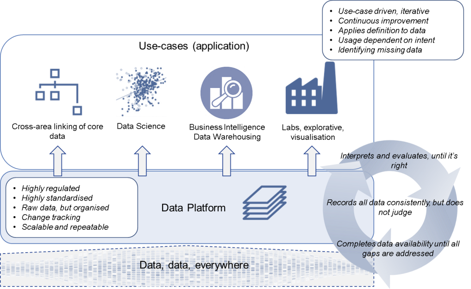
Next steps are to make sure we can connect information modelling and definitions (taxonomies, glossaries) to the graphs, so we can use these as the ‘steering wheel’ to guide the direction of our information and it’s management – illustrated by the image below. I want to be able to systematically / programmatically manage data integration through governance.

I have some time set aside to work on seeing how information modelling case-tools can be integrated into this thinking. Watch this space!

No more Batch ETL

A few weeks ago I wrote a post about the concept of having continuous execution of ETL individual processes to achieve ‘eventual consistency‘. In that post I made the case to step away from ‘Batch’ execution of ETLs, where related processes are executed as a mini workflow, in favour if fully independent execution of the individual (modular) ETL processes.

I have spend some time developing this concept in SQL Server using my VEDW Data Vault sample set and wanted to share some techniques how to achieve this.

It works even better than expected, if you have a SQL Server environment it’s worth checking out the code below. But the concepts are applicable for various architectures of course.

As a brief reminder, the ‘eventual consistency’ approach aims to remove all dependencies in loading data by allowing each individual ETL process (i.e. Hub, Link, Satellite) to run whenever possible – in a queue of sorts.

Enabling this requires a pattern change, for instance in the Data Vault example used here the ETLs  needed to be updated (=regenerated) to load from the Persistent Staging Area (PSA) using their own self-managed load window. This load window is set for every unique execution based on the committed data in the PSA (based on the ETL control framework, not the RDBMS).

The load windows between individual ETLs differ slightly as each ETL process runs at slightly different time, but this is no problem since you can derive the last moment consistency (Referential Integrity) was achieved using the control framework metadata. This information can be used for loading data into the next layer.

The setup – two continuous queues

What I want to achieve for this test is to have two separate ‘queues’ running continuously:

• One queue that loads new data (delta) into the Staging / Persistent Staging Area, and
• One that loads data into the Data Vault from the Persistent Staging Area.

As outlined above there are no dependencies managed between processes – the ETLs are required to ‘just work’ every time they are executed.

To up the ante a bit more, I want the first queue (PSA) to run more frequently and using more resources than the Data Vault queue.

I have tested this concept using SQL Server and SQL Server Integration Services (SSIS), and have generated the VEDW sample set as physical SSIS ETL packages (using Biml, of course). The generated packages have been moved (deployed) to an Integration Services Catalog (the default SSISDB was used). The result looks like this:

This screenshot shows a subset of the deployed packages in the SSIS catalog. In the ETL control framework I use (DIRECT) the workflows start with ‘b_’ (for ‘batch’) and the individual ETLs start with ‘m_’. (for ‘modular’). For all intents and purposes I have generated the ‘batch’ ones to run the Staging and Persistent Staging steps in one go, but arguably you can load into the PSA directly.

To keep things simple I will create one queue for the ‘batch’ packages (containing Staging and Persistent Staging), and another queue for all the Data Vault objects (prefixed by ‘m_200’).

Setting up a continuously running process queue for SSIS

Running something continuously, over and over again – almost as an ETL service, in SSIS isn’t straightforward. There is no out of the box option for this, but there is a trick to make this work (unless you want to invest in the message broker). An easy way to achieve this is to create a job in SQL Server Agent containing a single T-SQL step. The job can be configured to start when the server starts, it will keep running regardless as soon as you start it.

The T-SQL step is where the real process handling takes place and where the polling is implemented. The idea is to create an endless loop that:

• Checks if new ETLs can start based on parameters, and wait if this is not the case. The number of concurrent ETL executions is the parameter used in this example. If this is less than 3, the next ETL can be started according to a priority list (the queue). If there are already 3 (or more) ETLs running there will be a 30 second wait before new attempts are made.
• Execute the SSIS package that is next in line directly from the SSIS catalog using the corresponding T-SQL commands. The priority order is set by the queue, but in this example organised by last execution time. The jobs that haven’t been running for the longest will be prioritised in the queue.
• Handles exceptions to avoid the SQL statement to fail. This is implemented using a TRY…CATCH block that deactivates the ETLs in the control framework if there is an issue so they won’t be attempted again unless reactivated. An example use-case is when the queue attempts to execute a package which is not available in the package catalog (hasn’t been deployed).

Thanks Luciano Machado for the WHILE 1=1 idea!

The logic is as follows:

-- Create a temporary procedure to act as parameter input, i.e. calculate the number of active ETLs
CREATE PROCEDURE #runningJobs @NUM_JOBS int OUTPUT AS
(  
   SELECT @NUM_JOBS = (SELECT COUNT(*) FROM <ETL control framework> WHERE <execution status is 'running'>)
)
GO

DECLARE @MAX_CONCURRENCY INT
DECLARE @NUM_RUNNING_JOBS INT
DECLARE @DELAY_TIME VARCHAR(8)
DECLARE @JOBNAME as VARCHAR(256)
DECLARE @CURRENT_TIME VARCHAR(19)

SELECT @MAX_CONCURRENCY = 3
SELECT @DELAY_TIME ='00:00:30' -- This is the time the queue waits upon detecting concurrency

WHILE 1 = 1
BEGIN
  EXEC #runningJobs @NUM_RUNNING_JOBS OUTPUT

  --Whenever the number of jobs exceeds the parameter, wait for a bit (as per the delay time)
  WHILE (@NUM_RUNNING_JOBS >= @MAX_CONCURRENCY)
  BEGIN
    WAITFOR DELAY @DELAY_TIME
    EXEC #runningJobs @NUM_RUNNING_JOBS OUTPUT
  END
  -- When a spot becomes available, run the next ETL(s) from the queue
  SELECT TOP 1 @JOBNAME = ETL_PROCESS_NAME
  FROM
  ( -- Select the Module that hasn't run the longest (oldest age)
     SELECT *
     FROM <the queue>
  ) QUEUE
  ORDER BY <latest execution datetime> ASC

  BEGIN TRY -- Execute the ETL
    Declare @execution_id bigint
    EXEC [SSISDB].[catalog].[create_execution] @package_name=@JOBNAME, @execution_id=@execution_id OUTPUT, @folder_name=N'EDW', @project_name=N'Enterprise_Data_Warehouse', @use32bitruntime=False, @reference_id=Null
    Select @execution_id
    DECLARE @var0 smallint = 1
    EXEC [SSISDB].[catalog].[set_execution_parameter_value] @execution_id, @object_type=50, @parameter_name=N'LOGGING_LEVEL', @parameter_value=@var0
    EXEC [SSISDB].[catalog].[start_execution] @execution_id
  END TRY
  BEGIN CATCH
    <do something i.e. disable ETL in queue, send email etc.>
  END CATCH

  WAITFOR DELAY '00:00:05' -- A delayer to throttle execution. A minimum delay (1 second) is required to allow the systems to administer ETL status properly.
END
DROP PROCEDURE #runningJobs

When this is started, either directly as SQL statement or as part of a SQL Agent Job (T-SQL step) the process will keep on running until stopped.

Organising the queue

What about the queue itself? In its simplest form this can be a view that lists out the ETL packages that need to be executed, as long as the name corresponds with the name of the object in the SSIS catalog. At the very least the .dtsx suffix needs to be added as this is how package files are stored in SSIS.

The view I have used for this queries the ETL object names from the ETL control framework, as they need to be declared anyway for the control wrapper to work. In other words, the ETL names are already there. All I need is to select the most recent execution instance for each ETL I want to be in scope, so this can be listed in ascending order. This will force the ETL process that hasn’t run the longest will be put on top of the queue.

It becomes really easy to set up various queues as all it takes is a T-SQL statement and corresponding view (or other object). Creating the 2nd queue was a matter of seconds and in similar fashion a 3rd Data Mart queue can be configured.

The result

When executing the queues you can see the ETL process executions happening in the ETL control framework. I specifically started the Data Vault queue first to confirm no data would be loaded, which makes sense because the PSA was still empty. After a few minutes I started the Staging / Persistent Staging queue, and one by one (three at a time really due to the concurrency setting) the PSA tables were being populated. At the same time the Data Vault queue processes started picking up the delta, as soon as the PSA process for a specific table was completed succesfully.

With the queue being a view you can monitor the order change while processes are executed. An ETL process that was top off the list moves back to the bottom, and slowly makes its way back up again, as shown in the following screenshot:

It all works really well and after a while Referential Integrity was achieved. Also, the results were 100% the same as they were in the VEDW and Batch approaches. Making changes in the data were also picked up and propagated without any problems.

Final thoughts

The number of currently executing ETLs as used in the example here is a fairly crude mechanism. But, it is clear to see that this can easily be adjusted to more sophisticated resource management parameters such as CPU or memory usage. While I didn’t implement this for the example here, a queue should also have ways to validate completeness of ETL processes. This is relevant because previously the internal dependencies where safeguarded in the batch style mini workflows, but since the batch is gone you need other ways to make sure all required ETL processes are present.

The easiest way to apply checks like these is to validate if every Link or Satellite has corresponding Hubs relative to the (shared) source table. The same applies to Link-Satellites of course, which needs its supporting Link and it’s Hub ETLs to be present somewhere in the queue. You need to prevent having, say, a Satellite that is loaded from a specific source table without a Hub process that loads from the same table. This is nothing new – the same rules apply and the required metadata is already available. It’s just that enforcing these rules is slightly different in a queue.

‘The queue’ is a good concept and works really well. If you have a PSA (why wouldn’t you?) you may want to give it a go as the results surpassed my expectation.

As a nice side effect, it also makes re-inialisation super easy.  All you need to truncate your control table (or at least the relevant records) and the system does the rest to reload deterministically. Copying data is not needed anymore, and you can’t even make a mistake here because the patterns can re-process already loaded data without failure.

On top of this it also natively handles graceful completion of the ETL control framework wrapper because stopping the job doesn’t kill the SSIS package execution, it just prevents new processes from spawning. This means you can even put it on a schedule if you want the queue to operate only limited amounts of time. Win-win!

This is an example of how ‘eventual consistency’ can be implemented using SQL Server, and I recommend looking into it.

I receive a fair bit of questions on the Data Warehouse Virtualisation ideas and wanted to respond and discuss this via this post. I don’t have all the answer but can share my views and expectations.

When it comes to DWH Virtualisation and the Persistent Staging Area (PSA), the questions generally fall into two categories:

1. Isn’t it too slow? How about performance? Surely users don’t want to wait for hours to see results?
2. Why bother with Data Vault (or similar) at all? Can’t we just skip this or fall back on Kimball’s techniques? What value do we get from having an intermediate hyper-normalised layer?

What about performance?

If you have billions of billions rows of streaming data every second, virtualisation is not going to work (unless perhaps you have access to unlimited resources). I think this is fairly obvious. However when it comes to performance in general, and virtualisation / PSAs in particular, it is important to remember three things:

• Generally speaking it’s always about balancing ‘performance’ with ‘complexity’. The more performance is tuned, the more complex solutions tend to become – which comes with a maintenance overhead. Sometimes it works out better to sacrifice some performance in favour or simpler solutions.
• Not every solution uses ‘big data’. Many environments are relatively modest in size and can (still) have big business impact, and it wouldn’t be correct to assess concepts only from the perspective of the few big deployments. Scalability is important to understand and consider, but not everyone needs to adopt techniques to scale out to massive sizes.
• Last but most importantly, and in addition to the previous point, it is really all about flexibility and metadata management. If you can virtualise the various layers on top off a PSA – essentially having a logical Data Warehouse – it is relatively easy to switch between deployments and technical architectures. There is no lock-in and you can let the engine figure out how to best leverage various available and connected environments.

In other words, the argument that virtualisation doesn’t work because it does not perform in massive data sets is neither here nor there. The conversation should be how the concepts that are embodied in virtualisation / logical Data Warehousing can be supported in different environments so you can evolve with your technical infrastructure and requirements.

Metadata management and generation, in other words.

There are many ways to deploy the solutions, but the metadata is the same. The best example I can give is using the same metadata to create views (=virtualisation) and persist these (as either indexed / materialised views or physical ETL processes) if query times exceed certain thresholds. When this is not enough, the exact same metadata is used to move files to a MPP platform and interpreted using scalable (cloud) techniques.

With these techniques you can distribute processing everything over many nodes, calculate the result, move this into a cube and power everything down again (except the cube). I’m not saying this is the one-size-fits-all solution, but it can be the right one in some cases (with extremely low TCO).

These are real examples, which hopefully help to explain that purely creating views for virtualisation’s sake is not the end goal – the flexibility is.

Performance requirements are some of the ‘environmental parameters‘ that drive the deployment, how the engine decides how and what to generate!

What value do we get from having an intermediate layer?

Please consider this earlier post on how various concepts together support virtualisation and more.

When you are at the point that you have broken up all data integration components into tiny processes -which are all independent and allow for incremental extension of the data platform- and can throttle and distribute infrastructure resources (CPU, memory…) to rebuild everything from the raw original files / transactions (PSA)… Does it still make sense to develop a normalised core DWH layer (i.e. Data Vault)?

I have a lot of good things to say about Data Vault. For example I believe Data Vault has been instrumental in breaking up DWH techniques into modular components, enabling ETL generation and shaping the mindset that DWH systems need to be designed for change. I think it has a place in DWH architectures for some time to come, but that the focus shifts more from modelling discussions on what is basically a physical model towards becoming commodity components that are part of ‘the engine’ as outlined earlier.

This also means that conversations on hash keys versus business keys or ‘do we need Hubs or not’ are more and more irrelevant. Why? Because the physical implementation / these kinds of technical decisions can be driven from (design) metadata as well. This is fully in line with the Data Vault thinking, which for example defines a Hub as the embodiment of the business concept but doesn’t prescribe using hash keys or not…

I like the ‘unit of work’ style thinking and the natural ‘subject area’ definition of context related to a business concept (business key), and I think this abstraction assists in getting a better grip on information. I am placing my bets on improving conceptual / logical models that can be automatically generated as Data Vault models (for example) in the background with the optimal technical architecture fit.

I accept that this is level of design is not readily available yet, but it’s almost there.

My view is that there is no real intrinsic value in the layer itself, and focusing on the physical DWH model  – especially coming from a performance balancing point of view – as the core of the solution will experience diminishing returns. However, breaking up the architecture in layers helps in abstracting out complexity and consequently to keep things manageable. And as I mentioned a few times here we don’t necessarily design for these layers anymore.

The methodologies to date have assisted greatly in compartmentalising the various required concepts but should really be viewed as an engine that focuses on making things work, and as a stepping stone towards more advanced ways to define schema (taxonomies, glossaries).

If you imagine the inverse, for instance having a massive PSA with a Kimball-style Star Schema on top of this, I can imagine the complexities at enterprise scale. Well, not really just imagine because I did experience this in reality. I for one prefer having an abstraction layer to ‘put information in the right context’ first and applying logic a bit later.

Having said that, I use(d) to recommend smaller deployments to start this way, and consider adding an intermediate DWH core layer later (because the PSA supports this). But given the thinking outlines in this and previous posts this will also be absorbed by ‘the engine’.

What value do we get from having an intermediate hyper-normalised layer?

Let me start by stating that a Data Warehouse is a necessary evil at the best of times. In the ideal world, there would be no need for it, as optimal governance and near real-time multidirectional data harmonisation would have created an environment where it is easy to retrieve information without any ambiguity across systems (including its history of changes). Ideally, we would not have a Data Warehouse at all, but as an industry we have a long way to go before this can become a reality.

The other day I was discussing Data Warehouse architecture and collaboration topics during a phone conference and the following question was asked: ‘would it be worth to purchase any of the books on Data Vault (or similar hybrid modelling approaches)?’.

Apparently some of the book reviews were fairly negative by way of dismissing the Data Vault methodology as being past its prime. The question that came up during the call is one that is frequently recurring: would it still be worth investing time and energy in Data Vault or would time better be spend on working with, say, Python or Scala to directly develop data solutions given the current maturity of the industry?

Isn’t it just a hassle having to manage an additional Data Warehouse layer when you can directly code against the raw data?

Data Warehouse Virtualisation also appears to contribute to the idea that you don’t need a Data Warehouse (which I find a bit of a paradox). When you have ‘modularised’ all data integration components and can dynamically distribute infrastructure resources, rebuilding the Data Warehouse on the fly, does it still make sense to develop a normalised Data Warehouse layer with a technique such as a Data Vault? Can’t we just skip it?

I recently touched on this topic while addressing common questions in this post, but it’s worth exploring further. This is because there still seems to be is a ‘mindset gap’ between the ‘new’ world of ‘big data’ technologies and the more traditional world of developing Data Warehouse solutions on RDBMS technologies. And, the ‘new’ world often states it replaces the need for the ‘traditional’ one.

The opinion is sometimes that these worlds aren’t compatible, but my view is that there is no reason why this would be the case. They contain a mutually complementing set of skills and can greatly benefit from a unified approach.

To cut a long story short: my answer to the posed question would be that, no, Data Vault is not obsolete and will not be for a while as it has a role to play in this unified approach. This is also the case for similar hybrid modelling techniques. However, our thinking has evolved quite significantly over the last few years to the point that the first generation of books may not be accurately capturing the intent anymore.

Moreover, the core mechanics of data handling are increasingly pushed down into the background as a commodity – which is a decidedly different focus than physical data model design. Data Warehouse Automation software and frameworks such as BimlFlex (from Varigence, the creators of Biml), WhereScape and BIReady are continuously working towards this, as are my own (Github / collaboration) efforts on ‘Virtual Data Warehousing’.

In short: Data Vault seems destined to take a place in the technical delivery of data solutions, but less as a technique to design the data models. Data Vault has proven itself as a capable technique to support incremental, business focused and tightly scoped information delivery. It provides a strong foundation to base your designs on, but physical design itself should never be the focal point of data solutions. Information modelling and management should be.

Data Vault inherently is a technique for physical design, so it stands to reason it will take more of a back seat.

I refer to this thinking as ‘the engine’, which I have outlined earlier and will touch on a bit later in this article as well. The engine is the combination of design metadata (concepts, patterns, ETL generation mappings) and environmental metadata (infrastructure parameters and constraints) that decides and manages how the physical models and corresponding data integration logic (ETL – Extract, Transform and Load) are generated, and updated when required.

Design metadata covers for instance what the core business concepts and units of work are, while environmental metadata covers the infrastructural and technological constrains such as available integration technology (‘ETL tool’) or available cores, memory and disk space.

The engine relies itself on various underlying concepts which are explained in more detail in my previous post on these topics but are outlined in the diagram below for reference. The premise is always that you work towards a mechanism that easily lets you model information, while automatically refactoring the solution in the background. In technical terms, this covers things like automatically redefining physical tables and reloading these with data using automatically generated ETLs (and much more).

It is this view that supports unifying the ‘traditional’ and ‘new’ data worlds; after all, certain things need to be done on the raw data no matter what. Do we need a Data Warehouse layer for ‘Data Science’? Maybe not immediately and as a hard requirement, no, but it would be good if findings and data preparation outcomes would somehow be made available for other use cases. Similarly it is helpful if already curated information can be used directly as opposed to reinventing the wheel.

The essence and vision on the interlinking of data use-cases in the context of enterprise information management is clearly and succinctly captured in Ronald Damhof’s great Data Quadrant Model (read the article here, more information and generally on http://prudenza.typepad.com/). How can Quadrant IV effort be easily moved to Quadrant II?

This is what I’m exploring further here and this is where ‘the engine’, with its built-in Data Vault logic in the background, can assist.

An evolutionary view on Data Warehouse implementation

It seems that discussions on relevance of Data Vault often address very specific topics to make the case. For instance, ‘do we still need Hubs?’, ‘isn’t it better to create a separate table for each attribute?’ or ‘should I model this transaction as a Hub or a Link?’. These types of discussions are almost always focused on the physical implementation.

I look at using techniques such as Data Vault in an evolutionary way; how can we keep adapting the approach we use, keep the things that work in the current environments and move away from what doesn’t make sense anymore. Having a certain degree of atavism, where certain traits reappear after being away for a while, is fine too. It’s all about adapting to stay relevant in the context of your business.

There will always be some tension between the prescribed ways to use a certain technique, to be ‘compliant’ with an approach, and this kind of evolutionary thinking. By forcing yourself to stick to an implementation standard you will at some point reach its end of life (it will become extinct). However, by adopting a mindset of continuous improvement where the designs are altered on an ongoing basis, the chances of survival will greatly increase.

Data Warehouse Virtualisation as a concept is a good example of this. I use Data Vault concepts to deliver this, but the technical implementation itself has evolved significantly over time to meet new demands in both infrastructure and business use-cases. Ongoing evolution of the implementation now allows these techniques to span across (and using interchangeably) various different technical environments.  But, while the underlying raw information remains the same, the upstream delivery including the Data Vault model has changed many times.

Just to be clear: Data Warehouse Virtualisation does not mean that everything always needs to be 100% based on views, it’s the concept that changes in the model are directly and automatically translated into the required technology. It’s refactoring in the extreme: if you change your model, your data morphs with it. How? By using the updated metadata to either recreate views, or by dropping and recreating the (persisted) DWH target table and regenerating and executing the corresponding updated ETLs to populate the target table again.

Why would you want this? Isn’t the Data Warehouse model supposed to be relatively stable? My view is that this ideally would be the case, but that there is a maturity curve in play here. The early stages of implementation typically experience more volatility in the design, whereas in more mature environments – usually the ones with stronger information management & governance – the design tend to become increasingly stable. This is investigated in a bit more depth in an older post here, and of course varies from organisation from organisation.  Generally though, I don’t believe we can have all the wisdom upfront to make every (modelling) decision correctly – including defining the right core business concepts even in the most basic Raw Data Vault approach. Data Vault supports more iterative approaches that lead to gradual understanding, as such the ability to refactor becomes important.

A second, more technical way, to look at this is again from the engine perspective. Automated refactoring takes away having to think about physical design decisions such as splitting Satellites because a few attributes have a high change rate. The engine may decide to create many physical tables that correspond to a single bit of context for a business key, or not – or it may change every now and then dependent on data dynamics.

Data Warehouse Virtualisation in this context also allows for versioning of one or more components of the design. I even see opportunities to leverage concepts from the Enterprise Service Bus (ESB) and Service Oriented Architecture (SOA) world in terms of versioning the Data Warehouse outputs (canonicals??) based on underlying schema changes. Using Data Warehouse Virtualisation concepts it’s already feasible to host different versions of your Data Warehouse (or Data Marts) and allow subscribers of information to move to the newer version over a defined period of time.

Are we still talking about Data Vault in a physical sense? Not really; it’s more about core business concepts, their context and relationships (unit of work). In ‘the engine’ I introduced earlier, this will be translated into physical or virtual Hubs (or not) and a balanced set of Satellites and Links – as well as the corresponding logic (ETL) to refresh these, if required.

You could argue this is still Data Vault, but at a higher level of abstraction. This would be true, although we won’t be talking about Hubs, Links and Satellites anymore.

The point I am trying to make is that it’s not particularly meaningful to focus on the physical implementation if you are deciding if a technique such as Data Vault is worth adopting. Rather, my recommendation is to focus on managing the required metadata to support your data solution and enable ways to keep adapting, stay flexible.

In terms of the delivery itself; this should be subject to some form of meritocracy and reason. If it works in certain niches, it’s good. If you are following rules for the sake of it, that is not to anyone’s benefit. Recent discussions on hash keys versus natural keys fit in this context. There are many ways to look at this, why not pick the best delivery for the specific use-case?

From mechanics to model

It is worth considering this: a few (approximately 5-10) years ago we were documenting the patterns to deliver a scalable physical data model. Now, we have a solid grasp on the physical model and associated loading patterns (both ingestion and delivery), which means we don’t need to focus on the physical model as much anymore.

In other words, the mechanisms of the Data Vault patterns are becoming a commodity, and as a result can be automated and are losing visibility. They are being pushed ‘into the engine’ of data management. This does not mean that the concepts are no longer valid; it just means we will start accepting this as a standard and don’t need to think about them as much.

As I stated earlier, there seems to be little point arguing if a Hub needs to be persisted or whether we should use hashing or not. This can all be automated, so we have time for more value-added work such as additional emphasis on information modelling.

Spaghetti code

No matter what technology you have, there is no escaping the necessity to model information – to understand the concepts, relationships and behaviour of data.

In areas which heavily focus on outputs using raw data, which is common in the traditional Data Lake thinking, this often results in relatively large and complex code segments.  The code also needs to manage clean-up, rules and fundamental time-variance logic.

This very quickly results into a spaghetti-like mess of tangled code segments. This is one of the topics that Ronald Damhof touches on in the context of his Data Quadrant Model: how to move insights into a production state, so benefits can be realised on an ongoing basis (moving from Quadrant IV to Quadrant II).

I’m not saying it is wrong to pursue this arguably more explorative use of data. On the contrary, there is definitely value in this (which is also acknowledged as Quadrant IV in Ronald Damhof’s model). What I’m saying is that this does not replace the more structured management of data as is implemented in a Data Warehouse architecture.

In fact, it is quite easy to combine these. In my designs I have done so by incorporating the Persistent Staging Area (PSA) concept into the architecture.

Following this idea you can support both the explorative and structured ways of working with data, as is displayed in the diagram below (the Data Platform being the PSA):

As is often the case, technology is not the answer – but a flexible approach and proper metadata management is. I believe we will get the best overall outcome if we keep simplifying the way we can perform information modelling and continue to abstract out the ever-changing technical delivery.

Imagine you could quickly organise business concepts and context without having to worry about a physical model and create a point-in-time set around these core entities in a scalable environment. Having all the separations of concern built-int? Wouldn’t that be much easier to code against using Python for data science purposes (if that’s what works best for your specific use-case)?

I believe it would be, as a large amount of fundamental data management logic is already catered to, and any reusable logic can be ‘plugged-in’ the available set (technically for instance as a Business Data Vault object – but that is happening automatically in the background) – where it will be usable for other business areas, too.

This means we’re still using Data Vault, or equivalent hybrid techniques, but the patterns and ideas have blended in the background to enable simplification of design and development.

After having used Git(Hub) to work and collaborate on code for a long time, I have recently spent some time to merge and move various documentation artefacts to GitHub as well. This covers the Data Integration framework and Enterprise Data Warehouse (EDW) architecture documentation, most importantly the various Design Patterns and Solution Patterns. These patterns form the central body of content that actually try to explain how things work in practice.

I think it makes a lot of sense to use Github as a collaboration mechanism for documentation as well (i.e. not only for code). It’s just too time consuming to maintain various documentation sets in binary format (Word, PDF) as changes can’t be easily merged when you work across multiple teams and various geographical regions. Word has a great layout, but at the end of the day is a closed format that requires specific software to be used.

As a result, I have moved much of the documentation in the menu sections of this blog into a new documentation GitHub repository. Have a look at the collaboration section to get an idea of the scope of this, as well as an idea where to find it. The documentation on the blog pages in the menu, as well as many other artefacts in various other location have been merged.

As you can image, over time various small changes in some documents haven’t always been propagated to the others, and I found some of the earlier documents to be outdated. This is why I’m also in the process of re-reviewing and updating documentation where required.

GitHub is great for this, as it easily allows others to pick up some of the work and contribute as well. If people want to, they can even branch out specific parts of the content and take it into a different direction. True to the Git concept the solution with the most merit will ultimately survive because more people keep contributing to it. You can also use GitHub to keep track of issues and discussions around specific topics.

To really make this work the documentation will need to be in plain text (not Word) because this allows for diff views that highlight proposed changes – a sort of scalable change tracking. GitHub supports (it’s flavour of) MarkDown which is easy to use and doesn’t look too bad. You can also use (and/or embed) LaTex for this purpose if you use a lot of (math) formulas. From time to time you can choose to render ‘final’ versions as PDF, which doesn’t look that bad. With a bit of effort you can render this with corporate logos and things like that as well.

I’m aware of alternatives in this area, including things like Google Docs. But at the end of the day I’m a firm believer in the Git concept and see this as an effective way to continuously update documentation (across different teams and regions) and share this as well.

The DIRECT documentation (process control framework) has been moved to the DIRECT GitHub.

I’ve finally properly (I think) configured the website to allow registration and the adding of comments in a user-friendly way, without having the burden of endless spambots.

Registration, the creation of an account, will allow commenting and discussing content on the site itself which is a big improvement over the current email-based correspondence. After having the account setup you will receive a welcome email and be able to log in to the site using the login widget on the left panel.

Having the conversations via the site (as opposed to email) will share the feedback to the community and allow for broader discussions.

You can register by navigating to the ‘register to this site‘ menu option. I look forward to many constructive conversations on this forum!

Making hash keys smaller

A few months ago I posted an article explaining the merits of the ‘natural business key‘, which can make sense in certain situations. And, from a more generic perspective, why this is something the Data Warehouse management system (‘the engine‘) would be able to figure out automatically and change on the fly when required.

This article used the common approach of storing the hash values in character fields (i.e. CHAR(32) for MD5 and CHAR(40) for SHA-1), and the main feedback on the article has been that this is not the most efficient way to store hash values in a typical RDBMS. In other words, the difference between a 32 byte hash key and an integer natural business key is not always a fair comparison.

Instead, if the output of the hashing algorithm is stored in its raw (binary) form only half the bytes are required to achieve the same outcomes. This is an important thing to be aware of as it is likely to influence the decision, either by the designer or the ‘engine’ algorithm, to choose between hash keys or natural business keys.

More generally, adopting binary data types instead of character types for hash values is a significant improvement in the Data Warehouse design, because you effectively halve your storage on disk and double your I/O!

Typical storage behaviours

In a typical ‘by the book’ Data Vault solution (in my experience at least) the CHAR(32) hash keys amount to roughly half of the total volume of the complete solution, with Links being some of the biggest tables. From a physical point of view the Link tables are essentially tables that have mostly hash keys as attributes: the Link hash key and the individual Hub hash keys.

These tables are often larger than Satellites in terms of storage space. Satellites may contain more rows by virtue of the historisation but also compress better because of the denormalisation / redundancy. This is of course assuming some form of compression can be used, which depends on the available technical configuration and licensing.  Most people would agree that compression is a big impact improvement in any Data Warehouse environment considering CPU overhead versus I/O gains, so for these investigations this has been enabled.

These examples were created in a SQL Server environment and your mileage may vary. Hopefully though the above helps to paint the picture of how these technical decisions relate together. In any case there is a solid business case to switch to binary / raw storage of hash keys, and I recommend to adopt this if you haven’t done so already.

Raw and character hash keys

First, lets look at the classic / typical way to generate a hash key in SQL Server:

CONVERT(CHAR(32),HASHBYTES('MD5',ISNULL(RTRIM(CONVERT(NVARCHAR(100),[<Business Key>])),'N/A')+'|'),2)

What happens here is that the Business Key value is converted to a text type, converted to a binary hash value and lastly converted to character (CHAR(32)). The ‘2’ convert style essentially cuts off the first two characters of the initial binary output.

For example if we run the following code:

SELECT CONVERT(CHAR(32),HASHBYTES('MD5',ISNULL(RTRIM(CONVERT(NVARCHAR(100),'Roelant')),'N/A')+'|'),2)

The result would be C65BE84D225435AB4667DD5E8172DEDB.

If we run similar code, but without the conversion to CHAR(32) it looks as follows:

SELECT HASHBYTES('MD5',ISNULL(RTRIM(CONVERT(NVARCHAR(100),'Roelant')),'NA')+'|')

This has the output of 0xC65BE84D225435AB4667DD5E8172DEDB. Notice the difference of the initial two ‘0x’ characters.

It is perfectly doable to switch between the character and binary representations of the hash key in case you want to move towards a binary approach. Just convert it back to binary using the same style as was used before:

SELECT CONVERT(BINARY(16),'C65BE84D225435AB4667DD5E8172DEDB',2)

This will return the binary value that can be stored in the corresponding BINARY(16) data type: 0xC65BE84D225435AB4667DD5E8172DEDB.

As you can see, the character and binary types can be switched out which is good news for existing deployments. In most cases though (except virtualised solutions) this will require a rebuild of the ETL (to remove the CHAR conversion) and some scripts to apply the above changes to all tables. This is easy enough to develop though.

Final thoughts

The ideal data types for hash keys are based on the deterministic outcomes of the selected hashing algorithm:

• 16 bytes for MD5 (and earlier versions) – this would be 32 characters as string i.e. CHAR(32)
• 20 bytes for SHA1 / SHA – this would be 40 characters as string i.e. CHAR(40)
• 32 bytes for SHA2 – this would be a 64 byte character string i.e. CHAR(64)

You can easily check this by running a simple query such as this:

SELECT HASHBYTES('MD5', 'Roelant')

The hash representation is visible as 0x70DACD9612153FD11894B1F07F454217. If you then look at the storage requirement you can see this only takes up 16 bytes:

SELECT DATALENGTH(HASHBYTES('MD5', 'Roelant'))

This shows that the data storage is indeed 16 bytes. If we were to store this hash value as character we would store the value as text without the 0x leading value, which is again 32 characters.

In both the binary as the character configuration there is no need to use the variable type. Hash outputs are deterministic and will not vary in length, and not using a var type will save you two bytes per value. All these things add up in the Data Warehouse environments, so spending some time to further investigate this is a worthwhile investment.

Today, a new set of changes -all part of the ecosystem for Data Warehouse Automation– have been formally published as new releases on Github.

As always a large amount of work has been done in the background, and thanks go out to various projects and teams for providing input and suggestions.

This round of improvements concerns the TEAM (management of source-target mapping metadata) application, the Virtual Data Warehouse (VDW) pattern management tool and the Data Warehouse Automation class library (DLL).

What’s new?

The Data Warehouse Automation schema definition and class library (including the command-line utility, examples and validation features) has received an interesting tweak, courtesy of Martin Guenther, to load/map (deserialise) Json files regardless of their structure.

Previously, the Json files were required to match the structure of the Data Warehouse Automation schema. With this change any Json file can be consumed and, as long as there is a matching code generation pattern, can be used for whatever purpose and as such called from the command line or applications such as Virtual Data Warehouse.

If Json conformance to the schema definition is required, the validation calls can still be applies as part of this process.

For TEAM, a large number of bugfixes and usability improvements have been added including better handling of Data Object names that include schemas and reuse schema names that are set in the connection tabs.

Also, initial Presentation Layer examples are added. These were already available for VDW, but can now be generated from TEAM also. One cool feature is to right-click on the grid for a Presentation Layer object and generate the Json from there, something that will be rolled out across all types.

If you use this version, don’t forget to refresh the repository (Deploy Metadata Repository in the Repository screen). This will only rebuild components that are used for processing and will not remove metadata that has been entered by users – the repository can be rebuilt safely.

The Virtual Data Warehouse release contains some more quality-of-life fixes such as delays on the metadata refresh (this can consume the application when large amounts of metadata are refreshed), better logging and exception handling.

More visibly, some of the examples have been updated to match the changes in the Data Warehouse Automation definition (in the Dimension pattern).

Where can I find the latest version?

These latest releases can be found on Github, also including the detailed change log:

• TEAM v1.6.2. can be downloaded here.
• The Data Warehouse Automation solution can be downloaded here.
• Virtual Data Warehouse v1.6.4. can be downloaded here.

Today I spend some time finalising and testing new releases for the ecosystem for Data Warehouse Automation, specifically the Taxonomy for ETL Automation Metadata (TEAM) and the Virtual Data Warehouse (VDW) tools.

As a very brief recap, TEAM focuses on source-to-target mapping metadata, linking up a source object to a target object and generating a Json file conform the schema for Data Warehouse Automation.

VDW can ingest these files and apply these to patterns to generate ETL or code.

So, TEAM is the design metadata and VDW the code generator.

What has changed?

The latest versions (v1.6.3 for TEAM and v.1.6.5 for VDW) are primarily bug-fix and ease-of-use oriented based on project feedback from various implementations. The main changes for this release are:

• Added basic Data Vault validation, so that some issues related to table structure and convention mismatches are detected during validation.
• Hiding of features not used when in physical mode, so that the interface is cleaner.
• Added Json export features, including ‘next-up’ object in the lineage as relatedDataObject(s) and other related objects such as metadata connections.
• Removed the repository feature. This is meant to be ultimately deprecated and was only causing problems between versions for users. This is now always deployed as part of metadata activation.

Details on issues addressed are found in the (now closed) project for v1.6.3: https://github.com/RoelantVos/TEAM/projects/2.

A notable change that may have impact on existing implementations is the (improved) handling of prefixes and suffixes. This means that underscores ‘_’ are now not automatically added. Existing keys and prefixes may need updating as a result.

For example the key prefix SK or HSH may now need to be _SK or _HSH is the underscore needs to be retained. This is related to issue #73.

As always there are many smaller tweaks and tidy-ups such as additional documentation, hover-overs and UI improvements.

The VDW changes are mainly to support the pattern changes. These are not functional changes, but some patterns benefit from the ‘next up’ Related Data Object for lookup purposes. For example, the Staging Area patterns use this to support the Full Outer Join interface.

What are ‘logical’ deletes?

Recently I was engaged in a few (separate) conversations about the use of deleted flags, and I thought it may be beneficial to post a summary here.

A deleted flag, or indicator, is a special attribute that identifies if a record has been deleted from the originating operational (‘source’) system. This is referred to as a logical delete. The record may be physically deleted in the operational system, but the data solution preferably captures that this delete has occurred, and ‘flags’ this in the data.

In other words, the record is available in the data solution in its most current state, but labelled as a deleted record. This means that the data solution contains a history of events even though this information may no longer be available in the originating systems.

A deleted flag can be stored as a separate attribute, which is added to the record it refers to. However, in most cases this information is stored in a Change Data Capture (CDC) attribute.

This is because the mechanisms necessary to detect if a record has been physically deleted are built-in, or at least part of, CDC functionality. A change can be an insert, update or delete and this evaluation can be stored in a CDC attribute – making a separate deleted flag superfluous.

There are many ways how CDC can be implemented – how inserts / updates / deletes can be be detected. This post is not meant to go into this detail, but about why it is relevant to record this information – and when not to use it.

The important note to remember is that a CDC flag refers to the full row, as identified by its Primary Key. So, if the record is detected as ‘deleted’ this applies to the full record as it was in the originating system, and not a part of the record. We will need to be aware of this when we model the Integration Layer.

This view of defining CDC as a mechanism to detect new records, changed record or deleted records based on their original structure is a fairly narrow – though very useful – technical view. This is typically how CDC is implemented in the Staging Layer of the data solution, including the the Persistent Staging Area (PSA). In most cases, native CDC technologies provide the state of the record (i.e. all the values) at the time of delete so this creates a clear state of up to which point certain values were active.

CDC can also be defined as part of broader, more complex, approach to evaluate the correct context of Business Concepts / Business Keys (I will use these terms interchangeably in this post) in an information model or Integration Layer (e.g. Data Vault). This is the logic to define the correct state of a business concept (e.g. ‘Customer’, ‘Product’), including whether it should be considered active or not (at a point in time).

In this post, I refer to this line of thinking as ‘logical’ CDC, as opposed to the ‘technical’ CDC from the earlier paragraph. It is typically implemented in the Integration Layer of the data solution.

Why is having a deleted flag helpful?

In essence, recording logical deletes helps to guarantee that the data solution is in sync with what occurred in the operational systems from which the data was received. If we can’t detect that information is removed in these operational systems, how can we ensure that the information the data solution delivers is a correct representation?

A key success criteria for a data solution, at least in my opinion, is the ability to represent information as it appears (or appeared at some point in time) in the operational systems that provided the data. If you open up a screen in the operational system and view current clients, sales or customer details you would expect to see this information the same way in the reporting figures the data solution supports.

Recording CDC information, including logical deletes, supports the ability to do this. It its not the entire solution required to achieve this, but having access to logical deletes may be in some cases be necessary to evaluate the state of certain business concepts. This evaluation typically occurs in the Integration Layer, and is part of the ‘logical CDC’ concept.

Another interesting use-case is low level monitoring and even fraud detection. This is typically implemented in the Staging Layer; in the PSA.

A PSA simply records all incoming transactions ordered by their time of arrival in the data solution (the load date / time stamp). By storing the technical CDC information it is possible to query if certain records (keys to be precise) are removed from the system, or even added and removed multiple times.

It can be interesting to investigate why records are deleted, as it is often claimed that the application does not allow this. This is also true for common commercial applications.

It ‘should not happen’ that records are deleted, but sometimes somehow it still does and this may happen often.

Using the deleted flag to understand the state of a business concept

When determining the status (active or deleted) of a given business key in an Integration Layer (e.g. a Data Vault model), you cannot rely on (technical) CDC information alone.

Additional logic may be required to understand the impacts of the original CDC event on any specific attribute (the Business Key in this case), especially for a very denormalised source without any other context.

What I mean by this is that there may be no clear technical delete you can derive from just the CDC information, because this always applies to a full row based on the source Primary Key. And, in the Integration Layer, the Business Key may be different than the Primary Key of the original record.

If you would remodel the data, how would you determine for which columns the delete would apply and for which ones it doesn’t? In the Integration Layer this remodelling occurs often, because data is reorganised to conform to a defined information model – irrespective of how the original structure in which the data was stored.

Consider the image below, which shows the data in the original structure (‘source’) and how the data is remodelled in an Integration Layer (Data Vault) model. Natural Business Relationships (Links) are omitted for brevity. In this example the CDC mechanisms are able to evaluate the Change Data Operation for a given record, and this is recorded in the Staging Layer.

If a row with a delete comes though, what does this mean for the entities in the Integration Layer?

Granted, this is a pretty badly designed operational system. But then again, as data solution engineers we don’t always control the way the data can be made available. And the design between operational systems does vary, and by quite a bit.

I have experienced cases where a certain Business Concept wasn’t a key in the source system at all. It was always contextual to something else, similar to the ‘provider’ in the image here. In the Data Vault, we developed logic to evaluate if we consider this Business Concept active or not based on logical deletes in various related tables.

The more the source data set is denormalised, the less useful the logical delete will be for deriving the state of the Business Keys. This is because the row would contain more attributes, which are more likely to be spread out over many more Integration Layer entities and possibly populate various Business Concepts.

However, and this is why the logical CDC mechanisms are so much more elaborate than the technical CDC view, there is (much) more than just the logical delete flag to assert the state of a Business Key. Most systems have some sort of internal status or time stamp which is used to (functionally) determine if a Business Key is active or not. In these cases, this is much more valuable information.

Logical deletes do come in handy when this context is not available, and in these cases this can be stored in the Integration Layer as additional context for the Business Key. This could be done using a status tracking Satellite for example, or an equivalent Satellite that just contains an active / inactive flag.

Usually, the delete flag starts to diminish value quickly when you start moving data from the original record into their modelled counterparts. However, when the Business Key does align with the Primary Key in the operational system or when other context is lacking it still has its uses.

After many years I have finished up at Allianz to join the Varigence team, so that I can work on the BimlFlex solution for data solution automation.

Automating data solution has always been my long-term interest, and working for/with Varigence is an amazing opportunity to contribute to what is already a great suite of tooling. We’ll incorporate many ideas that are still ‘on the table’, and won’t lose sight of the open source community.

Working at Allianz group / Allianz Partners has been really great – and I hope to stay in touch with all the great people working there.

Last week I started at working for Varigence to work with the team on the BimlFlex solution for Data Warehouse Automation, so time to revisit some techniques in the Microsoft space.

While doing so, I re-created a lightweight approach for code generation and (data warehouse) automation that I really like and am sure can be useful in certain scenarios. It is one of many ways to get things done, and worth sharing as such.

Thanks go out to Komal Maurya for showing these capabilities.

This ETL/ELT generation & automation concept for Azure Data Factory (ADF) fits in the simple ETL generation series. This series contains a variety of similar-style approaches for getting started generating data logistics for your data solution, using templating (engines) and metadata input.

The same can be done for ADF, and in a very easy and (in my opinion) elegant way.

A setup for ADF Data Warehouse Automation

The approach is simple: ADF offers a ForEach activity (an object available in ADF) which essentially iterates of a collection (list) of items. For each item, it can perform one or more specified (sub)activities (invoked pipelines in ADF).

The convenient feature is that an item can be a complex object, such as a JSON structure. The example below shows this setup, where the ForEach object iterates over the items as available in the @pipeline().parameters.metadata object.

In this simple example setup, a ‘batch’ pipeline is created (displayed above) which calls another pipeline – called ‘pipeline_src_stg’.

The obvious question is: where does this ‘metadata’ object come from? This is defined as a parameter (or variable) at pipeline level.

This ‘metadata’ parameter is defined as an array, so something that can contain several items. As mentioned before an item can be a complex object, so it is possible to inject metadata in here that contains lots of information.

For this example, the array that is added here is as follows:

[
  {
    "runStgProcess": {
      "moduleCode": "exampleModule1",
      "sqlStatement": "SELECT Test FROM SourceTable",
      "targetTable": "TargetTable",
      "targetSchema": "dbo"
    }
  },
  {
    "runStgProcess": {
      "moduleCode": "exampleModule2",
      "sqlStatement": "SELECT SecondTest AS Test FROM SourceTableTwo",
      "targetTable": "TargetTable",
      "targetSchema": "dbo"
    }
  },
  {
    "runStgProcess": {
      "moduleCode": "exampleModule3",
      "sqlStatement": "SELECT Test FROM SourceTable",
      "targetTable": "TargetTableTwo",
      "targetSchema": "dbo"
    }
  },
  {
    "runStgProcess": {
      "moduleCode": "exampleModule4",
      "sqlStatement": "SELECT SecondTest AS Test FROM SourceTableTwo",
      "targetTable": "TargetTableTwo",
      "targetSchema": "dbo"
    }
  }
]

Basically, this JSON array (indicated by the square brackets) contains four separate data logistics processes (modules) each containing a SQL statement to retrieve the data and a target to load the results into. This is a simple example – but it can be extended to include additional properties, nested objects and basically anything that you have available in your metadata back-end.

If you are wondering where the SQL statement is coming from, please have a look at the corresponding paragraph near the end of this post for some background on this.

For now, this example loads records from two arbitrary sources into two arbitrary targets. Sources 1 and 2 go into target 1, and both sources are loaded into target 2 again also.

Inside the ForEach container

The activity called for each iteration is the invoked pipeline. In this pipeline, again at pipeline level, a parameter can be configured to ‘catch’ the value coming down from the original array in each iteration.

This is an object, which can be given the default value of @item() – an internal convention in ADF. An item() here is the object that is iterated over by the ForEach ADF activity.

To make this work, a parameter must be created at pipeline level for the pipeline_src_stg as displayed in the screenshot below.

This parameter can then be linked to the pipeline as invoked by the ForEach activity.

Now, in each iteration, the ‘metadata’ object receives an individual JSON segment from the original array. This information is now available in the pipeline and can be used everywhere in the activity, so that data can be moved around driven by the metadata.

Inside the (invoked) pipeline, a standard Copy Data activity has been created. This activity can be configured to accept dynamic sources and targets, which we can take from the metadata object (the item) that has been made available to the pipeline.

A generic connection for the ‘source’ has been created (a data set in ADF), which is configured to connect to the ‘source’ database. This source connection for the Copy Data activity can accept an object in addition to a straight-up SQL statement when we select the option to use a query as a source.

Objects can be added using the ‘add dynamic content’ option which becomes available if you click around in the query form.

In this case, because we want to make sure the SQL Statement property from the JSON input is used, we can add the following here object reference here: @pipeline().parameters.metadata.runStgProcess.sqlStatement.

This syntax follows the structure of the JSON input.

This way, we select the sqlStatement property from the runStgProcess object. The ‘metadata’ refers to the variable we have defined earlier to catch each individual JSON segment (item) in the invoked pipeline.

In other words, we specify that the source is a query but that the details of this query are passed on from the metadata object.

The configuration of the target is slightly more work because we have to configure additional parameters in the target data set for the table name and the schema name.

For the intended outcome, the table- and schema name must be taken from the metadata object as in the screenshot below. But to make these options available in the first place we need to define this as an option in the sink (target) dataset.

The values used are as follows, and as before these correspond to the property of the input JSON structure.

• @pipeline().parameters.metadata.runStgProcess.targetSchema
• @pipeline().parameters.metadata.runStgProcess.targetTable

To make these fields available, parameters can be defined for the dataset which is designated as the target. These are just string types as they will contain the corresponding string property from the JSON file.

And lastly, these local parameters can be assigned to the table name of the dataset.

Running the new process

At this stage, everything is in place to run the process with the input JSON content or file. For demonstration purposes the ForEach activity is configured to run each process sequentially, but in ADF this is configurable as well.

To run the process and input the metadata, the complete JSON can be inserted as input when the process is started.

This will open the monitoring console, where you can see that the information is passed to each iteration.

When the processes are finished (four iterations, as per the four JSON segments in the array), we can see the result in the database.

Success! Both sources are loaded to both targets as per the specified four modules.

Inputting the JSON metadata file

For this example we stored the JSON array as a parameter, and have the option to copy this into the parameter when we run the pipeline manually.

In ‘real’ deployments the JSON input can be provided as parameter or as a location to the JSON file in an accessible location such as an Azure Storage account (file storage).

Creating a pointer to a location where the metadata is maintained also helps as work-around on form limitations in the Azure portal, because there is a limit on the number of characters that can be added here. If you use a file location, all you need to do is update your JSON and continue running the processes – no updates in the ETL objects are needed.

Here you go, a fully generic SQL execution engine driven by input JSON metadata in ADF!

With this lightweight setup, you only configure ADF once. After this, everything can be metadata-driven.

Where does the SQL statement come from?

What has not been covered in this post is the creation of the JSON file itself. Generating a JSON file is not fundamentally different from generating SQL (or other) code in the same way this has been explained throughout this blog.

Examples include the simple ETL automation series and template-based code generation related to for example the Virtual Data Warehouse concept. The generic schema for Data Warehouse Automation also has many examples on how to generate this kind of output, including Data Vault examples and complex transformations.

The same approaches can be used to export your metadata in a JSON format that is defined in a way that matches with your ADF configuration. All you need is a good mechanism for managing your metadata, and potentially exposing this using the generic schema for Data Warehouse automation.

From here, it is easy to generate JSON files that can deliver real-world data solutions in various ways including this ADF example approach.

Final thoughts

This approach works well for solutions that look to push-down the compute into the database engine. Essentially, ADF is used as a scheduler and looks after the connectivity. All logic is executed against the selected database platform.

This is in many ways similar to approaches where templating engines are used to generate (complex) SQL, which is then executed against a given target platform. Data solutions using pattern-friendly methodologies such as Data Vault greatly benefit from this, and it is perfectly feasible to generate the entire solution this way. In fact, this has been done many times in real-world projects combining multiple and complex operational systems with large data sets.

The benefit is that ADF can be used to control the degree of parallelism and the connections. Many things can be parameterised in ADF, and when this is the case then metadata can be injected.

And in ADF, you can parameterise a lot.

If this makes sense to you, it may be worth checking out similar examples using DBT, the use of templating engines and of course the Virtual Data Warehouse.

The downside is that only generic configurations are used, and all logic is encapsulated in SQL. If you need a specific ADF object to do something different, you will need a separate component for this. Otherwise, all complex transformations are done in SQL, so your back-end must be able to generate this.

Another important note to make is that, for this to work, you need a mature metadata repository, catalog or framework so that you can manage your metadata in the first place – an important consideration to make between considering DIY and investing in vendor software.

This is where using BimlFlex comes in. Not only does BimlFlex has a complete metadata repository, but the platform allows you to specify metadata in a way that native components for data logistics can be generated for a number of supported target technologies (including ADF). This metadata, for this scenario, will then be generated as ADF objects such as complete pipelines, activities, lookups, data flows etc. using the Biml engine.

One of the things to ‘solve’ working for a software vendor is how to balance delivering meaningful content for the community for collaboration purposes with commercial software development and sales. We’re aligned that we want to make this work, so are continuing to discuss how we can do both.

The first action on this is the creation of a public Github repository that contains community-facing content that may be useful working with the Varigence toolset. This repository is the BimlFlex Community. It actually is a rebrand of an existing content, and we’ve tidied this up a bit so we have good content here as well as a place to publish things that may be useful to others going forward.

Of course, I will continue to work out and document concepts as I come across them as I have been doing for the last 10 years on this blog.

This is a verbatim of my presentation at Knowledge Gap 2021, about ways to collaborate on data warehouse automation.

In this presentation, I present the ideas and application of a schema that can be used to interface metadata between and across different delivery tools. Essentially, how we can use a generic schema to separate what we can agree on with what we don’t – and through this support all known data warehouse use-cases across different modelling techniques, patterns, and tools.

There is also a video available, either directly on YouTube or in the videos page on this blog. The repository covering this is found here on Github.

How to agree to disagree

There must be 1000s of code generation tools, scripts, accelerators, vendor platforms or tool add-ins focused on speeding up data warehouse delivery. Excel, SQL, code, more Excel. In fact, I only know a few people who have not been working on a tool of their own to use in their projects.

Delivering a good data solution, such as a data warehouse, is difficult and requires various concepts to play well together, and to be implemented correctly. With so many tools we have so many variations of the same theme, and some are better than others – or at least in certain areas. I am not sure we are always doing our projects, customers, and ourselves a favour by introducing yet another custom solution.

Developing data warehouses is not always easy. There are many options to evaluate, considerations to make, and frameworks to apply. When we design and deploy a data solution, we aim to integrate all these concepts and frameworks into a working coherent deliverable which ideally does everything as intended and also does it perfectly.

At the same time, we often work independently and in parallel on these complex topics – even when the projects we do can be very similar in nature. There has to be a way to exchange the common parts of our work, the design metadata, so that we can continue to make delivering data solutions easier and better, while everyone still gets to use the tools they like and are familiar with.

Design metadata is the information you need to generate your solution. By using such an approach, you may be able to save time re-inventing the wheel in various cases. At the same time, we can still continue to work with the same tools and patterns that we prefer.

Using an agreed format to exchange design metadata helps to allow you to focus on your core strengths. Some solutions have really great metadata management features, some are strong in modelling, some generate great code and some have really good control frameworks or conventions.

You may think, how can any generic schema be sufficient to store all the complexity I have in my solution; all the metadata I need to support my frameworks and automation? Actually, in most cases there is a ‘core’ of design information that is consistent across projects.

For example, in all cases data can go from A to B, or it is interpreted this way using a view or transformation (which I consider the same in this context). After various workshops and projects the schema is pretty stable, and it can always be adapted. There is also a concept of key/value pair extensions that was able to solve all specific requests so far without concessions made.

The approach is not tied to any specific technology or data modelling approach, and would support design metadata to build Dimensional Models, Data Vault, Anchor or 3NF. There is not anything that prevents a certain solution direction, and it’s up to you which parts you use and how you use them. In principle it’s also possible to relate different models together – for example, a mapping between conceptual to logical models.

If you are currently using a repository, that is compatible too. It’s relatively easy to write an adapter that can interface with a schema such as this. The added advantage is that the metadata can be stored in Json format, which is text based and easy to version control and share. This is usually easier than merging version in a database and lends itself well to DevOps. At the same time, having a separate artefact to merge into a repository is made easier by having a dedicated change file to process.

In some cases, the available automation tools work somewhat like a black box – sometimes requiring all data processing to be done internally behind the scenes. This sounds convenient, and it can be, but it also can force a lock-in using a concept, approach, or technology that you may not like as much. All is usually OK unless you want something different, and we’re still figuring things out in some areas.

Sometimes, these accelerators can be seen (usually by their creator – and I’m one of them) as worthy of strict IP protection.

Personally, I think the magic of automation is not really in the code generation but in the way we manage our design metadata. So let’s dive into the details.

Unboxing data warehouse automation

If you consider data warehouse automation as a black box, then the design metadata goes in and data logistics processes (artefacts) are generated and operated from there in some shape or form.

The idea behind the schema for data warehouse automation is to separate the management of the design metadata from its storage. Design metadata is the information you need to generate the files or database structures and the data logistics to interact with them.

Some tools do more than others, and often they do many things and have lots of knowledge embedded. From the perspective of metadata we can limit this to managing the design metadata, storing it, interfacing with it and applying some patterns against it for code generation. This is a separation of the way we work with the metadata from the way we store it and the way we use it.

When we look at it like this, we can start applying different technologies. For example, we could potentially use any tool we like to interact with the metadata. We can use our Excel sheets, our 3^rd party software, our homebrew (TEAM) or our favourite modelling tool. It doesn’t matter, because we read from and write to the same format.

We don’t need to align on technology to do our design, but we can work together on how we want to use this design metadata to deliver outputs. he same applies to design decisions on the ‘best’ way to deliver certain patterns. Do we need caching, do we need a lookup, do we need ETL or ELT?

We don’t need to agree on this. If we do, then great and if not we can just let the meritocracy play out. The design metadata is independent of this.

Data Objects, Items and Mappings

The schema for data warehouse automation is an open source project on Github. It has a number of components, such as a schema definition, documentation, a class library, some example metadata and patterns (in Handlebars) and a validation project.

The schema definition is a Json schema definition, which lists out the specifics of each segment. As a Json file, it can be consumed in various ways – some of which are explained in the project on Github.

The schema defines what I refer to as a Data Object, which can be a file, query, table or container. Whatever it is. A Data Object can have Data Items, which can be attributes or queries again.

In a simple implementation a Data Object is a table and a Data Item is a column, and you can have mappings between one Data Object to another as well as for their Data Items.

This mapping between on Data Object and another is a Data Object Mapping.

It brings together a source Data Object to a target Data object with some properties (such as the classification and filter criteria displayed) and optionally includes a lower-level Data Item Mapping as well. In practical terms, the Json definitions from the schema are instantiated as it they were classes in traditional object oriented programming.

The result is a very easy and practical way to create all kinds of data structures, data logistics or transformations ranging from very simple to extremely complex.

I have prepared a few examples of text-based code generation using this approach on Github, but it works the same way if you’re using SDKs, APIs or 3^rd party compilers such as Biml.

Need more?

One feature I would like to highlight is way you can attach an extension to each definition, at every level. If there’s something specific you need, you can always create an extension for this. This is basically a key/value pair with a description, and it can be applied everywhere.

Let’s work together!

This is a high level introduction of why a schema for data warehouse automation could make sense, and how it works. This schema can facilitate collaboration without forcing us into a certain solution or technology corner. It an open source project on Github that includes documentation, a class library, a validation technique and various regression testing scripts and samples.

The schema works by separating design metadata management from storage, and provides a simple and flexible way we read from, and write to, design metadata. If you have an automation tool, or are developing one, please have a look at what is already available and how we can work together.

If you don’t, you may miss out on connecting your solution to other frameworks and evolving concepts. However, if you do, you may find you can focus on your specific area of interest, your strength, more because some of the other necessary concepts can be reused.

I genuinely feel that approaches such as these are in the best interest of ourselves and the projects we deliver. If we can at least agree on the basics, we don’t have agree on the way we use the design metadata. That will work itself out naturally. We do not have to agree on the best way to implement x, y or z – we can discuss and let the meritocracy play out. But at least we can hopefully agree that fundamentally we are all mapping data from A to B somewhere.